Unit 5 · Lesson 5.3
Autoencoders for anomaly detection
Lesson 4.2 scored records by how badly a few principal components reconstruct them. An autoencoder generalizes that idea. It is a neural network trained to reproduce its input through a narrow intermediate layer, and when it is trained on normal traffic, the error with which it reconstructs a new record serves as an anomaly score. This lesson defines the architecture, shows that a linear autoencoder learns nothing beyond PCA, examines what reconstruction error does and does not measure, describes Kitsune, a network intrusion detector built from autoencoders, and compares an autoencoder with an isolation forest on the course data under an alert budget.
Architecture and training
An autoencoder consists of an encoder \(f\) that maps an input \(x \in \mathbb{R}^d\) to a code \(u = f(x) \in \mathbb{R}^q\) and a decoder \(g\) that maps the code back to a reconstruction \(\hat{x} = g(u) \in \mathbb{R}^d\). Both are neural networks, typically MLPs as in Lesson 5.1. When \(q < d\), the code layer is a bottleneck, and the network cannot simply copy its input; it must keep the information that best explains the training data. Training minimizes the average reconstruction loss, usually the squared error,
by mini-batch gradient descent with backpropagation, exactly as for a classifier, with the input serving as its own target. No labels are needed in the loss. Labels enter through the choice of training data. For anomaly detection the autoencoder is trained on records believed to be normal, and the reconstruction error \(e(x) = \lVert x - \hat{x} \rVert^2\) of a new record is its anomaly score.
Figure 5.6 shows the network of Lab 5b. It takes the eleven standardized flow features of Lab 4, passes them through a hidden layer of 32 ReLU units to a code of 3 numbers, and mirrors this in the decoder. It is trained for 60 epochs with Adam on the normal records of days 0 to 7, and its loss is monitored on the normal records of days 8 and 9.
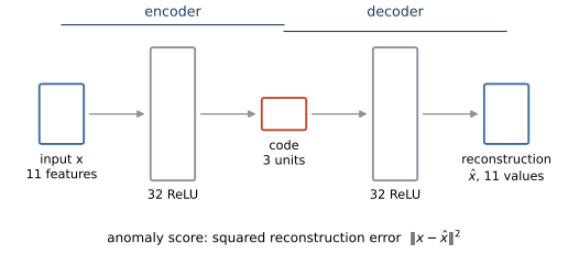
Figure 5.6. The autoencoder of Lab 5b. The encoder maps 11 standardized flow features through 32 ReLU units to a code of 3 numbers; the decoder maps the code through 32 ReLU units back to 11 values. Box heights indicate layer widths. The anomaly score of a record is the squared Euclidean distance between the input and its reconstruction.
A linear autoencoder is PCA
Remove the nonlinear activations, and the encoder and decoder are affine maps, so the whole network computes an affine map of rank at most \(q\) (the collapse of stacked linear layers shown in Lesson 5.1 applies). Baldi and Hornik (1989) analyzed this case for squared error. When the data covariance matrix is invertible and its eigenvalues are distinct, the error function has, up to an invertible change of the code, a unique local and global minimum, at which the network's overall map subtracts the mean, projects orthogonally onto the subspace spanned by the first \(q\) principal components (the leading eigenvectors of the covariance matrix) and adds the mean back; all other critical points are saddle points, not local minima. Because there are no other local minima, gradient descent on a linear autoencoder usually ends near the PCA reconstruction of Lesson 4.2. It learns the subspace, not the individual components. Any invertible linear transformation of the code, undone by the decoder, gives the same reconstruction, so the code units need not be orthogonal or ordered by variance.
In the worked example of Lesson 4.2, a linear autoencoder with a one-number code, trained on the five records, would learn to project onto the line through (3, 3) in the direction (1, 1), reconstruct the new record (4, 2) as (3, 3), and give it a reconstruction error of 2.0, the same value PCA gives.
Lab 5b checks the result on the course data. A linear autoencoder with a three-number code, trained with Adam, reaches a validation error of 0.3459 per feature, against 0.3456 for three principal components fitted to the same records. The principal angles between the subspace spanned by its decoder and the PCA subspace are all below 1.1 degrees, so the two subspaces nearly coincide. Depth does not change this. A linear autoencoder with many layers is still an affine map of rank at most \(q\), and its optimum is still the PCA projection. To go beyond PCA the network needs nonlinear activations, which let it reconstruct data lying near a curved surface rather than a flat subspace.
With ReLU activations, the autoencoder of Lab 5b reaches a validation error of 0.1034 per feature, much lower than PCA's 0.3456 with the same code size. It models normal traffic better. Whether it detects attacks better is a different question.
Show the answer
Without activation functions every layer is affine, and their composition is a single affine map whose rank is at most 3, the width of the narrowest layer. By the result of Baldi and Hornik, the best such map under squared error is the projection onto the subspace of the first three principal components (after centering), so after successful training the network reproduces three-component PCA. The extra layers add parameters, not expressive power. It is neither nonlinear nor an extension of PCA; it is PCA with redundant parameters and a slower, iterative fit.
Reconstruction error is a heuristic
The use of reconstruction error as an anomaly score rests on an assumption. Because the network was trained only on normal records, it should reconstruct normal records well and anything different poorly. The error therefore measures how far a record departs from the structure the network has learned from the normal training data, that is, the part of the record that the network cannot reproduce. It is not a definition of an anomaly, and it is certainly not a definition of an attack. The assumption fails in three ways, each of which matters in security.
First, an autoencoder can reconstruct some anomalies well. Gong et al. (2019) observe that the assumption that anomalies produce higher reconstruction error does not always hold, and that an autoencoder sometimes generalizes so well that it can also reconstruct anomalies well; they proposed adding a memory module to limit this. A network with enough capacity learns a general-purpose compression of anything resembling its training data, including attacks that differ from normal traffic only in combinations it can still represent.
Second, benign records that are new produce high errors. A new backup schedule, a software update that changes connection patterns, or a new branch office all generate traffic the autoencoder has not seen. Sommer and Paxson (2010) stress that anomaly detectors report what has not been seen before, whether benign or not. Networks drift, so a model trained last month raises errors on this month's normal traffic unless it is retrained.
Third, attacks designed to look normal, or that happen to, produce low errors. In the course data a share of every attack family was generated with its features blended toward the benign behavior it imitates, and the command-and-control family c2beacon consists of small, regular connections that resemble web browsing.
Figure 5.7 shows the outcome on the test days. The median error is 0.72 for normal records and 2.41 for attacks, so attacks do tend to be reconstructed worse. The two distributions overlap over most of their range, however.
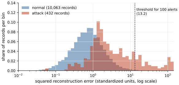
Figure 5.7. Squared reconstruction error (log scale) of the Lab 5b autoencoder on the test records of days 10 to 13, normal (blue) and attack (red), each normalized to sum to 1 over the bins so that the two classes can be compared despite their different sizes. The dashed line is the threshold that yields 100 alerts over the four days. Most attacks lie below it, and the records above it include normal ones.
Setting the threshold from an alert budget
A threshold turns the error into alerts. A common recipe is to take a high percentile of the errors on normal training data, or their maximum. Kitsune, described next, uses the largest error observed during training as its basic threshold. Such rules fix the false positive rate on the training data, and therefore depend on the most extreme normal records seen in training and on how the error distribution shifts afterwards. They leave the alert volume uncontrolled. The alternative of Lesson 4.3 is to rank records by error and alert on the top \(k\), with \(k\) set by the alert budget, or to set the threshold at the \(k\)-th highest error of a recent period of the same length.
Lab 5b takes a budget of 100 alerts over the four test days and sets the threshold at the 100th highest test error, 13.2. (Ranking the test period's own scores is legitimate here because a top-\(k\) rule needs no labels; in daily operation you would rank each day's records or carry over the previous period's threshold.) At this threshold only 0.20% of normal test records are flagged, the precision of the alerts is 0.80, and the recall is 0.19, because 81% of the attacks fall below the threshold. A false positive rate that small, applied to about ten thousand normal records, still supplies a substantial share of the alerts, the base-rate effect of Lesson 1.2 once more.
Kitsune
Mirsky et al. (2018) built Kitsune, a network intrusion detector that learns without labels and runs online. A feature extractor maintains incremental statistics of each network channel over damped time windows, so that memory stays small. A feature mapper groups the features into small subsets. KitNET, the detector, then uses an ensemble of small three-layer autoencoders, one per subset, each reporting its root mean squared reconstruction error, and an output autoencoder that learns the normal pattern of those errors and produces the final score. It is trained on traffic assumed to be normal during an initial training mode. The authors argue that an ensemble of small autoencoders is more efficient than a single autoencoder over the whole feature space, and they report detection performance comparable to offline anomaly detectors on their evaluation, even on a Raspberry Pi.
Kitsune's threshold illustrates the point of the previous section. In its basic form the threshold \(\varphi\) is the largest score seen during training, and an alert is raised when a score reaches \(\varphi\beta\) for a sensitivity parameter \(\beta \ge 1\). The authors also suggest fitting a distribution to the training scores and alerting on improbable values, and they leave the choice to the user. Both options depend on the training mode being free of attacks. Traffic in an operational network during the first hours of deployment is not guaranteed to be clean, and anything present then is learned as normal.
Autoencoder or isolation forest
An isolation forest (Lesson 4.3) is an ensemble of random trees and has nothing in common with a neural network except that both turn normal training data into an anomaly score. They are worth comparing for that reason. Lab 5b trains both on the same normal records of days 0 to 7 with the same eleven features. Figure 5.8 summarizes the results. The autoencoder reaches an AP of 0.366, the isolation forest 0.387 and three-component PCA 0.323, against 0.598 for the supervised MLP of Lesson 5.2 and a test base rate of 0.041. The autoencoder's far better reconstruction of normal traffic yields a modest gain over PCA and no gain over the forest.
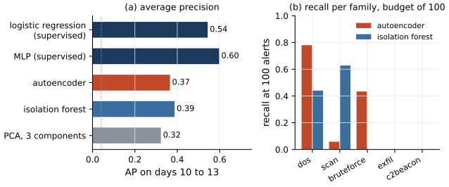
Figure 5.8. Detectors on the test days of Lab 5b. (a) Average precision of two supervised detectors (logistic regression and the MLP of Lesson 5.2, trained with labels) and three detectors trained on normal records only (the autoencoder, an isolation forest and reconstruction error from three principal components); the dotted line is the base rate. (b) Recall of each attack family among the 100 highest-scored test records for the autoencoder and the isolation forest.
Panel (b) shows that the two unsupervised detectors find different attacks. At the budget of 100 alerts the autoencoder finds 78% of the denial-of-service records and 43% of the brute-force attempts but 6% of the scans, while the isolation forest finds 63% of the scans, 44% of the denial-of-service records and 0% of the brute-force attempts. Neither finds any exfiltration or command-and-control records within the budget. Their overall precision at the budget is similar (0.80 and 0.76). An autoencoder measures departure from the learned structure of normal records in every feature at once, and the forest measures how easily a record is separated by random splits on single features, so the two notions of unusual select different records. Combining detectors, or giving each a share of the budget, is a reasonable response; replacing one by the other on the strength of a single AP is not.
Show the answer
These records would become training data, the network would learn to reconstruct them and similar records, and their errors would fall, so most of them would drop out of the top 100 and be replaced by other records. That is how a detector adapts to benign drift, and some periodic retraining is necessary. The risk is that the training data now includes whatever attacks were not detected in that period, including the command-and-control traffic, and the autoencoder learns to reconstruct them too. Retraining on unreviewed data turns undetected attacks into normal behavior. Sommer and Paxson list a related weakness among the well-recognized problems of anomaly detection, that attackers can evade detection by gradually teaching a system to accept malicious activity as benign. Retraining should use reviewed data or, where that is not possible, should at least exclude the alerts an analyst has not cleared and the records that scored just below the alert threshold.
Practical notes
Standardize the inputs, with the statistics of the normal training records, so that every feature contributes to the error on the same scale; otherwise the error is dominated by whichever feature has the largest variance. Choose the code size and the number of epochs on a validation period of normal records that follows the training period, and remember that a much lower reconstruction error need not give a much better detector, as the comparison with PCA showed. Keep the per-feature errors as well as their sum, because they tell an analyst which features made a record unusual, which is the beginning of an explanation. And evaluate the detector the way it will be used, with precision and per-family recall at the alert budget on a later period than the training data.
Lab 5b
A neural detector and an autoencoder
Open in ColabRead with outputsNotebook on GitHubAbout 2 minutes to run on a laptop CPU
Summary
An autoencoder compresses its input through a bottleneck and reconstructs it, and trained on normal records it scores new records by their reconstruction error. With linear activations and squared error its optimum is the projection of the centered data onto the leading principal subspace, as Baldi and Hornik showed, so only nonlinear activations take it beyond PCA; Lab 5b confirms that a linear autoencoder learns nearly the PCA subspace. Reconstruction error is a heuristic. Autoencoders can reconstruct some anomalies well, benign novelty and drift raise errors, and attacks that resemble normal traffic stay below any useful threshold, which the overlapping score distributions of the lab make visible. Kitsune shows how small autoencoders can serve an online network detector, with a threshold taken from training scores; a threshold set from the alert budget controls the alert volume instead. On the course data the autoencoder models normal traffic far better than PCA but ranks attacks about as well as an isolation forest, and the two find different attack families.
References
- Baldi, P., and Hornik, K. (1989). Neural networks and principal component analysis: Learning from examples without local minima. Neural Networks, 2(1), 53-58. https://doi.org/10.1016/0893-6080(89)90014-2
- Gong, D., Liu, L., Le, V., Saha, B., Mansour, M. R., Venkatesh, S., and van den Hengel, A. (2019). Memorizing normality to detect anomaly: Memory-augmented deep autoencoder for unsupervised anomaly detection. 2019 IEEE/CVF International Conference on Computer Vision (ICCV), 1705-1714. https://doi.org/10.1109/ICCV.2019.00179
- Mirsky, Y., Doitshman, T., Elovici, Y., and Shabtai, A. (2018). Kitsune: An ensemble of autoencoders for online network intrusion detection. Network and Distributed System Security Symposium (NDSS 2018). https://doi.org/10.14722/ndss.2018.23204
- Sommer, R., and Paxson, V. (2010). Outside the closed world: On using machine learning for network intrusion detection. 2010 IEEE Symposium on Security and Privacy, 305-316. https://doi.org/10.1109/SP.2010.25