Unit 5 · Lab 5a
Backpropagation by hand, then in PyTorch
Lab 5a
Backpropagation by hand, then in PyTorch
Open in ColabRead with outputsNotebook on GitHubAbout 1 minute to run on a laptop CPU
# On Google Colab, install the scikit-learn version the course was built with.
# On your own computer, install requirements.txt instead; this cell then does nothing.
import subprocess, sys
if "google.colab" in sys.modules:
    subprocess.run([sys.executable, "-m", "pip", "install", "-q", "scikit-learn==1.9.0"], check=True)
Lab 5a. Backpropagation by hand, then in PyTorch
This lab computes the gradients of a tiny neural network three ways and checks that they agree, then trains a slightly larger network by gradient descent and watches its decision boundary form. It runs in well under a minute on a laptop CPU.
You will:
- implement the forward pass, the loss and the backward pass of the 2-2-1 network of Lesson 5.1 in NumPy;
- check every gradient against finite differences;
- check it again against PyTorch's automatic differentiation (autograd);
- apply one gradient-descent update and confirm that the loss falls;
- train a 2-16-1 network on an XOR-like problem for a few hundred steps and plot the decision boundary as it trains.
import os

import numpy as np
import matplotlib.pyplot as plt
import torch

torch.set_num_threads(4)
torch.manual_seed(0)
np.set_printoptions(precision=6, suppress=True)
1. The worked example
The network has two inputs, two hidden ReLU units and one sigmoid output. With input \(x\) and label \(y \in \{0, 1\}\) (here \(y = 1\), an attack), the hidden pre-activations are \(z = Wx + b\), the hidden activations are \(h = \max(0, z)\), the output pre-activation is \(a = v^\top h + c\), the predicted probability is \(p = \sigma(a)\), and the loss is the binary cross-entropy \(\ell = -[y \ln p + (1-y)\ln(1-p)]\). The parameter names and values are those of Lesson 5.1.
x = np.array([1.0, 2.0])
y = 1.0
params = {
    "W": np.array([[0.5, -0.2], [0.3, 0.4]]),
    "b": np.array([0.1, -0.1]),
    "v": np.array([0.6, -0.5]),
    "c": np.array(0.2),
}
lr = 0.5

def sigmoid(a):
    return 1.0 / (1.0 + np.exp(-a))

def forward(p, x, y):
    z = p["W"] @ x + p["b"]
    h = np.maximum(0.0, z)
    a = p["v"] @ h + p["c"]
    prob = sigmoid(a)
    loss = -(y * np.log(prob) + (1 - y) * np.log(1 - prob))
    return {"z": z, "h": h, "a": a, "p": prob, "loss": loss}

cache = forward(params, x, y)
for k, v in cache.items():
    print(f"{k:<5} {v}")
z [0.2 1. ] h [0.2 1. ] a -0.18 p 0.45512110762641994 loss 0.7871917248407819
2. The backward pass
The chain rule, applied from the loss back toward the inputs, gives each gradient from the one computed just before it. For a sigmoid output with cross-entropy loss, \(\partial \ell/\partial a = p - y\).
def backward(p, x, y, cache_):
    g = {}
    da = cache_["p"] - y                 # dL/da
    g["v"] = da * cache_["h"]            # dL/dv = dL/da * h
    g["c"] = np.array(da)                # dL/dc
    dh = da * p["v"]                     # dL/dh
    dz = dh * (cache_["z"] > 0)          # ReLU passes the gradient only where z > 0
    g["W"] = np.outer(dz, x)             # dL/dW[j, i] = dL/dz[j] * x[i]
    g["b"] = dz
    return g, {"da": da, "dh": dh, "dz": dz}

grads, inter = backward(params, x, y, cache)
for k, v in inter.items():
    print(f"{k:<3} {v}")
for k, v in grads.items():
    print(f"dL/d{k}:\n{v}")
da -0.5448788923735801 dh [-0.326927 0.272439] dz [-0.326927 0.272439] dL/dv: [-0.108976 -0.544879] dL/dc: -0.5448788923735801 dL/dW: [[-0.326927 -0.653855] [ 0.272439 0.544879]] dL/db: [-0.326927 0.272439]
3. Check against finite differences
For each parameter \(\theta\), the central difference \([\ell(\theta + \epsilon) - \ell(\theta - \epsilon)]/(2\epsilon)\) approximates \(\partial \ell/\partial\theta\) with a truncation error of order \(\epsilon^2\). We use \(\epsilon = 10^{-6}\), so this term is of order \(10^{-12}\). In double precision each loss value also carries a rounding error of about \(10^{-16}\), and the division by \(2\epsilon\) magnifies it to about \(10^{-10}\). This rounding error sets the size of the difference printed below.
def numeric_grad(p, x, y, eps=1e-6):
    out = {}
    for k, v in p.items():
        gk = np.zeros_like(v, dtype=float)
        for idx in np.ndindex(v.shape):
            plus = {kk: vv.copy() for kk, vv in p.items()}
            minus = {kk: vv.copy() for kk, vv in p.items()}
            plus[k][idx] += eps
            minus[k][idx] -= eps
            gk[idx] = (forward(plus, x, y)["loss"] - forward(minus, x, y)["loss"]) / (2 * eps)
        out[k] = gk
    return out

num = numeric_grad(params, x, y)
fd_max_diff = max(float(np.max(np.abs(num[k] - grads[k]))) for k in params)
print(f"largest |analytic - finite difference|: {fd_max_diff:.2e}")
largest |analytic - finite difference|: 1.28e-10
4. Check against PyTorch autograd
PyTorch records the operations of the forward pass and runs the chain rule backward through them when loss.backward() is called. We repeat the forward pass in double precision and compare.
tp = {k: torch.tensor(v, dtype=torch.float64, requires_grad=True) for k, v in params.items()}
xt = torch.tensor(x, dtype=torch.float64)
z_t = tp["W"] @ xt + tp["b"]
h_t = torch.relu(z_t)
a_t = tp["v"] @ h_t + tp["c"]
loss_t = torch.nn.functional.binary_cross_entropy_with_logits(a_t, torch.tensor(y, dtype=torch.float64))
loss_t.backward()
torch_max_diff = max(float(np.max(np.abs(tp[k].grad.numpy() - grads[k]))) for k in params)
print(f"loss in PyTorch: {loss_t.item():.10f}   in NumPy: {cache['loss']:.10f}")
print(f"largest |NumPy gradient - autograd gradient|: {torch_max_diff:.2e}")
loss in PyTorch: 0.7871917248 in NumPy: 0.7871917248 largest |NumPy gradient - autograd gradient|: 0.00e+00
5. One gradient-descent step
Backpropagation has produced the gradient; it has not changed any weight. The update is a separate step, here plain gradient descent with learning rate 0.5, \(\theta \leftarrow \theta - 0.5\,\partial \ell/\partial\theta\).
new_params = {k: params[k] - lr * grads[k] for k in params}
for k, v in new_params.items():
    print(f"{k}:\n{v}")
after = forward(new_params, x, y)
print(f"loss before {cache['loss']:.4f}, after {after['loss']:.4f}; p before {cache['p']:.4f}, after {after['p']:.4f}")
W: [[0.663464 0.126927] [0.16378 0.127561]] b: [ 0.263464 -0.23622 ] v: [ 0.654488 -0.227561] c: 0.47243944618679007 loss before 0.7872, after 0.2624; p before 0.4551, after 0.7692
6. Training on an XOR-like problem
No straight line separates the two classes below. Points in the first and third quadrants are class 1, and points in the second and fourth are class 0. A logistic regression, which can only draw a line, does little better than chance on such data, but a network with one hidden layer can do much better. The data is synthetic, drawn with a fixed seed.
The code generalizes the backward pass above to a batch of \(N\) points and \(H = 16\) hidden units. The loss is the mean cross-entropy over the batch, so every gradient is an average over points.
rng = np.random.default_rng(5)
N, H = 400, 16
X = rng.uniform(-1, 1, size=(N, 2))
Y = (X[:, 0] * X[:, 1] > 0).astype(float)
flip = rng.random(N) < 0.05            # 5% label noise
Y[flip] = 1 - Y[flip]

net = {
    "W": rng.normal(0, np.sqrt(2 / 2), size=(H, 2)),   # He initialization for ReLU, fan-in 2
    "b": np.zeros(H),
    "v": rng.normal(0, np.sqrt(1 / H), size=H),
    "c": np.array(0.0),
}

def batch_forward(p, X):
    Zh = X @ p["W"].T + p["b"]
    Hh = np.maximum(0.0, Zh)
    A = Hh @ p["v"] + p["c"]
    return Zh, Hh, A, sigmoid(A)

def batch_loss_grad(p, X, Y):
    Zh, Hh, A, P = batch_forward(p, X)
    eps = 1e-12
    loss = -np.mean(Y * np.log(P + eps) + (1 - Y) * np.log(1 - P + eps))
    dA = (P - Y) / len(Y)
    g = {"v": Hh.T @ dA, "c": np.array(dA.sum())}
    dZ = np.outer(dA, p["v"]) * (Zh > 0)
    g["W"] = dZ.T @ X
    g["b"] = dZ.sum(axis=0)
    return loss, g

# The batch gradient agrees with autograd at the initial weights.
loss0, g0 = batch_loss_grad(net, X, Y)
tn = {k: torch.tensor(v, dtype=torch.float64, requires_grad=True) for k, v in net.items()}
At = torch.relu(torch.tensor(X) @ tn["W"].T + tn["b"]) @ tn["v"] + tn["c"]
lt = torch.nn.functional.binary_cross_entropy_with_logits(At, torch.tensor(Y))
lt.backward()
xor_torch_diff = max(float(np.max(np.abs(tn[k].grad.numpy() - g0[k]))) for k in net)
print(f"initial loss {loss0:.4f}; largest difference from autograd {xor_torch_diff:.2e}")
initial loss 0.6787; largest difference from autograd 4.16e-17
STEPS, LR = 600, 0.5
snap_steps = [0, 50, 150, 600]
gx = np.linspace(-1.1, 1.1, 61)
GX1, GX2 = np.meshgrid(gx, gx)
grid = np.column_stack([GX1.ravel(), GX2.ravel()])
snapshots, losses, accs = {}, [], []
for step in range(STEPS + 1):
    loss, g = batch_loss_grad(net, X, Y)
    losses.append(float(loss))
    accs.append(float(((batch_forward(net, X)[3] > 0.5) == Y).mean()))
    if step in snap_steps:
        snapshots[step] = batch_forward(net, grid)[3].reshape(GX1.shape)
    if step < STEPS:
        for k in net:
            net[k] = net[k] - LR * g[k]
print(f"loss: step 0 {losses[0]:.3f}, step 150 {losses[150]:.3f}, step {STEPS} {losses[-1]:.3f}")
print(f"training accuracy: step 0 {accs[0]:.3f}, step {STEPS} {accs[-1]:.3f}")
print(f"share of points whose label was flipped: {flip.mean():.3f}")
loss: step 0 0.679, step 150 0.341, step 600 0.322 training accuracy: step 0 0.598, step 600 0.930 share of points whose label was flipped: 0.055
fig, axes = plt.subplots(1, len(snap_steps), figsize=(12, 3), sharey=True)
for ax, s in zip(axes, snap_steps):
    ax.contourf(GX1, GX2, snapshots[s], levels=[0, 0.5, 1], colors=["#dbe6f1", "#f3d9d2"])
    ax.contour(GX1, GX2, snapshots[s], levels=[0.5], colors="k", linewidths=1)
    ax.scatter(X[Y == 0, 0], X[Y == 0, 1], s=6, c="#3B6E9E")
    ax.scatter(X[Y == 1, 0], X[Y == 1, 1], s=6, c="#C0492C")
    ax.set_title(f"step {s}, loss {losses[s]:.3f}")
plt.tight_layout()
plt.show()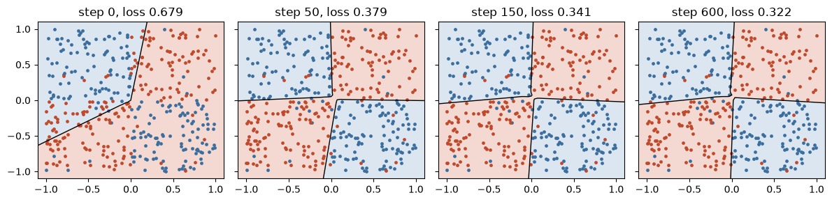
At step 0 the boundary is wherever the random initialization put it. It bends toward the quadrant structure as training proceeds. The training accuracy stays below 1 because some labels were flipped on purpose (the cell before the plot prints their share); even the exact quadrant rule misclassifies them.
Try this
- Change the hidden ReLU to the identity, both in
batch_forwardand in its derivative(Zh > 0)inbatch_loss_grad(replace the mask by 1), so the network becomes a stack of affine maps. Predict the training accuracy after 600 steps, then run it. - Set the learning rate to 5.0 and then to 0.05. What happens to the loss curve in each case?
- In the worked example, change
bto[-0.6, -0.1]so that the first hidden unit is inactive. Which gradients become exactly zero, and why?
Results summary
results = {
    "z1": float(cache["z"][0]), "z2": float(cache["z"][1]),
    "a": float(cache["a"]), "p": float(cache["p"]), "loss": float(cache["loss"]),
    "da": float(inter["da"]),
    "dv_1": float(grads["v"][0]), "dv_2": float(grads["v"][1]), "dc": float(grads["c"]),
    "dh1": float(inter["dh"][0]), "dh2": float(inter["dh"][1]),
    "dW_11": float(grads["W"][0, 0]), "dW_12": float(grads["W"][0, 1]),
    "dW_21": float(grads["W"][1, 0]), "dW_22": float(grads["W"][1, 1]),
    "loss_after": float(after["loss"]), "p_after": float(after["p"]),
    "fd_max_diff": fd_max_diff, "torch_max_diff": torch_max_diff,
    "xor_torch_diff": xor_torch_diff,
    "xor_n": N, "xor_hidden": H, "xor_steps": STEPS, "xor_lr": LR,
    "xor_loss_start": losses[0], "xor_loss_end": losses[-1],
    "xor_acc_start": accs[0], "xor_acc_end": accs[-1],
    "xor_flip_share": float(flip.mean()),
}
for k, v in results.items():
    print(f"{k:<16} {v}")

export = {
    "X": np.round(X, 4).tolist(), "Y": [int(v) for v in Y],
    "grid": np.round(gx, 4).tolist(),
    "snap_steps": snap_steps,
    "snapshots": {str(s): np.round(snapshots[s], 4).tolist() for s in snap_steps},
    "losses": [round(v, 5) for v in losses], "accs": accs,
}

# When the course build runs this notebook, it saves the numbers for the lesson pages.
if os.environ.get("COURSE_RESULTS"):
    import json
    with open(os.environ["COURSE_RESULTS"], "w") as f:
        json.dump({"results": results, "data": export}, f)
z1 0.19999999999999998 z2 1.0 a -0.18 p 0.45512110762641994 loss 0.7871917248407819 da -0.5448788923735801 dv_1 -0.10897577847471601 dv_2 -0.5448788923735801 dc -0.5448788923735801 dh1 -0.32692733542414804 dh2 0.27243944618679006 dW_11 -0.32692733542414804 dW_12 -0.6538546708482961 dW_21 0.27243944618679006 dW_22 0.5448788923735801 loss_after 0.2624328050465342 p_after 0.7691780475152374 fd_max_diff 1.283089190451392e-10 torch_max_diff 0.0 xor_torch_diff 4.163336342344337e-17 xor_n 400 xor_hidden 16 xor_steps 600 xor_lr 0.5 xor_loss_start 0.6787316263182898 xor_loss_end 0.3215969186180909 xor_acc_start 0.5975 xor_acc_end 0.93 xor_flip_share 0.055