Unit 5 · Lesson 5.2
Training neural networks in practice
Backpropagation supplies the gradient, and turning it into a trained detector requires a series of further choices. How many records contribute to each step, how large the step is and how it changes over time, where the weights start, how the features are scaled, how the network is kept from memorizing its training data, and how the rare class is weighted all change the model that comes out. This lesson covers these choices in the order you meet them when you train a detector, illustrates most of them with Lab 5b on the course dataset, and points out where scikit-learn's MLPClassifier differs from a network written in PyTorch. The textbook of Goodfellow, Bengio and Courville (Goodfellow et al., 2016) covers the optimization, initialization and regularization topics in more depth and is the background reference for this lesson.
Epochs, mini-batches and iterations
The training loss is an average over \(N\) training records. Computing its exact gradient at every step is expensive and, for large \(N\), unnecessary. Mini-batch stochastic gradient descent (SGD) shuffles the training records, splits them into batches of \(B\) records, and takes one step per batch using the gradient of the loss averaged over that batch,
where \(\theta\) is the vector of all weights and biases, \(\ell(x_i, y_i; \theta)\) is the loss of record \(i\) with features \(x_i\) and label \(y_i\) (Lesson 5.1), \(\eta > 0\) is the learning rate and \(\mathcal{B}\) is the current batch. Each step is an iteration, and one pass over all \(N\) records is an epoch. Because the last batch of an epoch is smaller when \(B\) does not divide \(N\), an epoch has
not \(N/B\). With \(N = 1{,}000\) and \(B = 64\), for example, an epoch has 15 full batches and one batch of 40 records, 16 iterations. In Lab 5b the fitting period has \(N = 21,056\) records and \(B = 256\), so every epoch has 83 iterations. The noise in \(\hat{g}\) shrinks as \(B\) grows, and in exchange for it each step costs far less computation than a full-batch step. Because the number of iterations per epoch depends on \(B\), plots of loss against epochs are easier to compare across batch sizes than plots against iterations.
Momentum and Adam
Plain SGD moves along the current gradient only. Momentum accumulates a velocity across steps. Rumelhart et al. (1986) already used it, in the form
where the momentum coefficient \(\mu \in [0, 1)\) determines how much of the previous step is kept. Along a direction where successive gradients agree, each step grows to about \(1/(1-\mu)\) times a plain gradient step, ten times for \(\mu = 0.9\); along a direction where they alternate in sign, successive contributions partly cancel and each step shrinks to about \(1/(1+\mu)\) of a plain step.
Adam (Kingma and Ba, 2015) keeps exponentially decaying averages of the gradient and of its elementwise square and scales each parameter's step by them. With \(g_t\) the gradient at step \(t\), \(\alpha\) the step size, \(m_t\) and \(v_t\) the running averages of the gradient and of its square, \(\beta_1, \beta_2 \in [0, 1)\) their decay rates, \(\epsilon\) a small constant that prevents division by zero, and all operations elementwise,
with \(m_0 = v_0 = 0\). The divisions by \(1 - \beta_1^t\) and \(1 - \beta_2^t\) correct the bias of averages that start at zero. Kingma and Ba give \(\alpha = 0.001\), \(\beta_1 = 0.9\), \(\beta_2 = 0.999\) and \(\epsilon = 10^{-8}\) as good defaults for the problems they tested. One consequence is easy to check by hand. At the first step, \(m_1 = 0.1\, g_1\) and \(v_1 = 0.001\, g_1^2\), so the corrected averages are \(g_1\) and \(g_1^2\), and every parameter with a nonzero gradient moves by almost exactly \(\alpha = 0.001\) in the direction opposite to its gradient, whatever the gradient's size, provided it is much larger than \(\epsilon\). Adam's step sizes are set by \(\alpha\) more than by the scale of the gradients, and Goodfellow et al. note that it is generally regarded as tolerant of the choice of its hyperparameters, although the learning rate sometimes needs to be changed from the default.
Adaptive methods are not uniformly better. Wilson et al. (2017) constructed a linearly separable problem on which gradient descent and SGD reach zero test error while AdaGrad, RMSProp and Adam reach test errors arbitrarily close to one half, and in experiments with several deep learning models they observed that the solutions found by adaptive methods generalized worse, often significantly worse, than those of SGD, even when they had better training performance. The practical rule is to treat the optimizer as a hyperparameter and compare candidates on a validation set, not on the training loss.
Panel (b) of Figure 5.4 trains the same network from the same initial weights on the course data with three optimizers. After 30 epochs, the training loss is 0.0211 for SGD with learning rate 0.1, 0.0213 for SGD with momentum 0.9 and learning rate 0.01, and 0.0086 for Adam with its default learning rate, with test AP of 0.598, 0.593 and 0.598. Adam reaches by far the lowest training loss and the lowest validation loss (0.0290, against 0.0383 and 0.0371), yet the three test APs are close. A lower loss did not produce a better ranking here, which is the reason to compare optimizers on the metric you will report. This is one run of untuned settings on one dataset, so it says nothing about which optimizer is better in general.
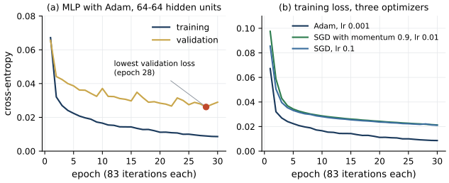
Figure 5.4. Training curves of the MLP of Lab 5b (22 inputs, two hidden layers of 64 ReLU units, one output), fitted on days 0 to 7 with mini-batches of 256 records. (a) Training and validation cross-entropy per epoch with Adam; the validation set is days 8 and 9, and the red point marks the epoch with the lowest validation loss. (b) Training cross-entropy per epoch for three optimizers started from the same initial weights.
Learning rate and schedules
The learning rate needs particular care. Goodfellow et al. (2016) describe the symptoms of a poor choice. If it is too large, the learning curve shows violent oscillations, with the cost often increasing significantly; if it is too low, learning proceeds slowly and can become stuck at a high cost. A schedule changes the rate during training, typically starting larger and decreasing. Goodfellow et al. note that a sufficient condition for SGD to converge is that the rates \(\eta_k\) satisfy \(\sum_k \eta_k = \infty\) and \(\sum_k \eta_k^2 < \infty\), and that in practice it is common to decrease the rate linearly until some iteration and keep it constant afterwards. Step schedules that divide the rate by a constant every few epochs, and schedules that reduce it when the validation loss stops improving, follow the same logic. They advise choosing the rate by monitoring learning curves of the loss over time. In Lab 5b every optimizer uses a constant rate, which is enough to see the differences.
Initialization
The initial weights must break symmetry. Two hidden units with the same activation, connected to the same inputs, that start with identical weights receive identical gradients and remain identical forever, so random initialization is required. Goodfellow et al. call this perhaps the only property of initialization known with complete certainty. The scale matters too. If weights are too large, activations and gradients grow from layer to layer; if too small, they shrink. Glorot and Bengio (2010) proposed drawing the weights of a layer with \(n_j\) inputs and \(n_{j+1}\) outputs uniformly from \(\pm\sqrt{6}/\sqrt{n_j + n_{j+1}}\), so that the variances of activations and back-propagated gradients stay roughly constant across layers. For ReLU units, which set every negative pre-activation to zero and so keep exactly half of the mean square of a zero-mean symmetric input (the quantity that sets the variance of the next layer's pre-activations), He et al. (2015) derived a zero-mean Gaussian with standard deviation \(\sqrt{2/n_l}\), where \(n_l\) is the number of inputs to the layer, and set biases to zero. PyTorch's nn.Linear uses its own default, drawing weights and biases uniformly from \(\pm 1/\sqrt{n_{\text{in}}}\), which is what Lab 5b uses. Lab 5a uses the He scale for the hidden layer of its XOR network.
Standardize the features
Gradient descent uses one learning rate for all weights. If one input is a byte count in the millions and another a rate between 0 and 1, the gradients of their weights differ by orders of magnitude, and no single learning rate suits both. A rate small enough to keep the large-scale weights stable leaves the others almost frozen. Standardizing every feature to mean 0 and standard deviation 1, after a log transform of heavy-tailed counts (Lesson 2.1), puts all inputs on the same scale. The scaler is fitted on the training data only, like every learned preprocessing step. In scikit-learn the safe way is a pipeline, which also guarantees that the same scaling is applied at prediction time:
import warnings
import numpy as np
from sklearn.datasets import make_classification
from sklearn.exceptions import ConvergenceWarning
from sklearn.neural_network import MLPClassifier
from sklearn.pipeline import make_pipeline
from sklearn.preprocessing import StandardScaler

warnings.filterwarnings("ignore", category=ConvergenceWarning)
X, y = make_classification(n_samples=5000, n_features=20,
                           weights=[0.97], random_state=0)
# one feature on a much larger scale, like a byte count
X[:, 0] *= 1e6

model = make_pipeline(
    StandardScaler(),  # fitted on the training data inside the pipeline
    MLPClassifier(hidden_layer_sizes=(64, 64), alpha=1e-4,
                  batch_size=256, random_state=0,
                  max_iter=30),  # counts epochs for adam and sgd
)
model.fit(X, y)
mlp = model[-1]
print(len(mlp.loss_curve_), "values in loss_curve_, one per epoch")
updates = mlp.n_iter_ * int(np.ceil(len(X) / 256))
print(mlp.n_iter_, "epochs,", updates, "weight updates")
The snippet prints 30 values in loss_curve_ and 600 weight updates, 30 epochs of \(\lceil 5{,}000/256 \rceil = 20\) iterations. Two details of MLPClassifier are easy to misread. For the stochastic solvers (adam, the default, and sgd), max_iter is the maximum number of epochs, not of weight updates, and loss_curve_ holds one value per epoch, the average training loss over that epoch, so it should be plotted against epochs. A training loss computed this way also includes the L2 penalty described next.
Show the answer
\(21{,}067/512 \approx 41.15\), so each epoch has \(\lceil 41.15 \rceil = 42\) iterations, 41 full batches of 512 and a last batch of \(21{,}067 - 41 \times 512 = 75\) records. Forty epochs perform \(40 \times 42 = 1{,}680\) updates. Truncating \(N/B\) to 41 would undercount by one update per epoch, 40 updates in all.
Overfitting and regularization
A network with tens of thousands of weights can memorize a training set of a few hundred records, driving the training loss toward zero while the loss on new data rises. Lab 5b provokes this deliberately. It trains a network with two hidden layers of 256 units (71,937 parameters) on 600 records of the fitting period, which contain 19 attacks, for 200 full-batch epochs, and measures the loss on the validation days after every epoch. Figure 5.5 shows the result. The training loss falls to 0.0008. The validation loss reaches its lowest value, 0.0537, at epoch 53 and then climbs to 0.0874 by the last epoch.
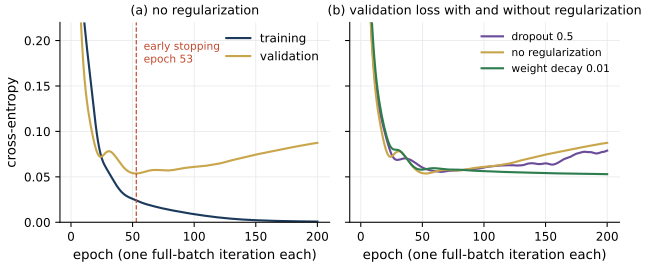
Figure 5.5. A network with two hidden layers of 256 ReLU units trained full-batch with Adam on 600 records of days 0 to 7 (Lab 5b); each epoch is one iteration. (a) Training and validation cross-entropy per epoch without regularization, with the epoch of lowest validation loss marked (early stopping). (b) Validation cross-entropy without regularization, with weight decay 0.01, and with dropout of probability 0.5 after each hidden layer. The validation set is days 8 and 9 in every case.
Early stopping keeps a copy of the weights whenever the validation loss improves and returns the best copy at the end. Goodfellow et al. (2016) describe it as probably the most commonly used form of regularization in deep learning, popular for its effectiveness and simplicity. In the lab it returns the weights of epoch 53, whose validation loss is far below that of the final weights. Their test AP, however, is 0.526, against 0.553 for the final weights. A plausible explanation is that the later epochs make some validation scores confidently wrong, which cross-entropy punishes heavily, while the order of the scores, which is all AP measures, kept improving. Early stopping on cross-entropy optimizes the loss; if the detector will be judged by its ranking, stop on a ranking metric computed on the validation period instead. The validation data must be separate from both the training and the test data, and for security data it should come after the training data in time, as days 8 and 9 do here.
L2 regularization adds \(\tfrac{\lambda}{2} \lVert \theta \rVert^2\) to the loss, and weight decay shrinks every weight by a constant factor at each step. The two are equivalent for plain SGD and differ for Adam, as this section shows. The penalty's gradient adds \(\lambda \theta\) to the gradient at every step, so plain gradient descent becomes
which shrinks every weight by the factor \(1 - \eta\lambda\) before the usual step, for example by 0.999 per step when \(\eta = 0.1\) and \(\lambda = 0.01\). For SGD, adding the penalty to the loss and shrinking the weights are therefore the same thing. Loshchilov and Hutter (2019) showed that L2 regularization and weight decay are equivalent for standard SGD (after rescaling by the learning rate) but not for Adam, where the penalty's gradient is divided by the same running scale as the loss gradient. They proposed applying the decay separately from the adaptive step, the method available in PyTorch as AdamW. The weight_decay argument of PyTorch's Adam, used in Lab 5b, adds \(\lambda\theta\) to the gradient, which is the L2 form. With \(\lambda = 0.01\), the validation loss in panel (b) no longer climbs in the later epochs; its minimum, 0.0529, comes at epoch 200 of 200, and the final training loss stays at 0.0278 instead of approaching zero.
Dropout (Srivastava et al., 2014) temporarily removes units, with their connections, at random during training, sampling a new thinned network for each presentation of each training case, so the network cannot rely on any particular unit. Srivastava et al. retain each unit with probability \(q\) during training and multiply the outgoing weights by \(q\) at test time, so that the expected input to the next layer is the same in both phases. PyTorch's nn.Dropout takes the drop probability \(1 - q\) as its argument and scales the kept activations by \(1/q\) during training, so nothing changes at test time; model.eval() switches dropout off. With a drop probability of 0.5, the lab's validation loss falls to 0.0554 at epoch 65 and then rises again, to 0.0789 by the last epoch, so dropout alone does not prevent the late rise of the validation loss.
Read the test AP alongside the curves for the other two runs as well. The early-stopped AP is 0.526 without regularization, 0.517 with dropout and 0.517 with weight decay, although weight decay gives the lowest validation loss. Cross-entropy measures both the order of the scores and how confident they are, while AP depends only on the order. A plausible reading is that weight decay keeps the scores from becoming overconfident, which lowers the loss without improving the order. A regularizer that improves the loss need not improve the ranking a detector is judged by, which is why the selection criterion should be the metric you will report.
Scikit-learn's MLPClassifier offers L2 regularization through alpha (the penalty is divided by the number of samples in the mini-batch before being added to the loss) and early stopping through early_stopping=True. It has no dropout. Its early stopping also holds out a random, stratified fraction of the training data (validation_fraction), not the most recent records, so on time-ordered security data the validation set it chooses is mixed into the training period. For a temporal validation split, train for a fixed number of epochs and select on your own validation period, or use PyTorch as Lab 5b does.
Class imbalance and weighted loss
Attacks are rare in the training data, 515 of 21,056 records in the lab's fitting period. The cross-entropy averages over records, so the normal records dominate the gradient. A weighted loss multiplies the cross-entropy of each attack record by a weight \(w_+ > 1\), where \(y \in \{0, 1\}\) is the label and \(p = \sigma(a)\) the predicted probability of attack for logit \(a\) (Lesson 5.1),
which PyTorch's BCEWithLogitsLoss provides as pos_weight. Setting \(w_+\) to the ratio of normal to attack records, 39.9 in the lab, makes the two classes contribute equally in total. The effect is easy to misjudge. The weighted network's test AP is 0.604, against 0.598 without weighting, so the ranking barely changes. What changes is the meaning of the output. At a threshold of 0.5 the unweighted network raises 211 alerts on the test days with precision 0.99 and recall 0.48, and the weighted one raises 288 alerts with precision 0.83 and recall 0.55. Weighting moves the predicted probabilities upward for everything that resembles an attack, which acts much like lowering the threshold, and it leaves probabilities that are no longer calibrated for the true base rate (Lesson 2.3). If the operating point is chosen from an alert budget, weighting is rarely needed; if it is chosen by a fixed probability threshold, weighting and threshold must be chosen together.
Show the answer
For a normal record (\(y = 0\)) the weighted loss is \(-\ln(1 - p)\), unchanged, so the gradient is still \(p\). For an attack record (\(y = 1\)) the loss is \(-40 \ln p\), whose derivative with respect to \(a\) is \(-40(1 - p) = 40(p - 1)\), forty times the unweighted \(p - y\). Each attack therefore pushes the weights forty times as hard as before, which shifts the scores of attack-like records upward.
The lab's detector
Panel (a) of Figure 5.4 shows the training and validation curves of the full MLP on the 21,056 fitting records. The validation loss is lowest at epoch 28 of 30, so with this much data and this network early stopping hardly changes anything. At that epoch the MLP reaches a test AP of 0.598, against 0.543 for logistic regression trained on the same records and features. Among its 100 highest-scored test records it finds 0% of the command-and-control records, a family it has never seen. Here the extra flexibility helps with attack types present in the training data and does nothing for the type that is absent from it.
Lab 5b
A neural detector and an autoencoder
Open in ColabRead with outputsNotebook on GitHubAbout 2 minutes to run on a laptop CPU
Summary
An epoch is one pass over the training data and has \(\lceil N/B \rceil\) iterations of mini-batch SGD. Momentum accumulates steps along consistent directions, and Adam scales each parameter's step by running averages of the gradient and its square, which makes its step sizes depend on \(\alpha\) more than on the scale of the gradients, although in the experiments of Wilson et al. its solutions sometimes generalized worse than those of SGD. The learning rate and its schedule are chosen from learning curves, initialization must break symmetry at a scale that keeps signals stable across layers, and features must be standardized, inside a pipeline, after log-transforming heavy-tailed counts. Early stopping on a validation period that follows the training period, L2 weight decay (which for Adam differs from decoupled decay) and dropout all counter overfitting, and their benefit should be judged with the metric the detector will be evaluated on. In scikit-learn's MLPClassifier with the stochastic solvers (adam, the default, and sgd), max_iter counts epochs, loss_curve_ has one value per epoch, and regularization is limited to alpha and early stopping. Weighting the loss for rare attacks mostly moves the scores, so it matters for a fixed probability threshold and little for a threshold set from an alert budget.
References
- Glorot, X., and Bengio, Y. (2010). Understanding the difficulty of training deep feedforward neural networks. Proceedings of the Thirteenth International Conference on Artificial Intelligence and Statistics, PMLR, 9, 249-256. https://proceedings.mlr.press/v9/glorot10a.html
- Goodfellow, I., Bengio, Y., and Courville, A. (2016). Deep Learning. MIT Press. https://www.deeplearningbook.org
- He, K., Zhang, X., Ren, S., and Sun, J. (2015). Delving deep into rectifiers: Surpassing human-level performance on ImageNet classification. 2015 IEEE International Conference on Computer Vision (ICCV), 1026-1034. https://doi.org/10.1109/ICCV.2015.123
- Kingma, D. P., and Ba, J. L. (2015). Adam: A method for stochastic optimization. 3rd International Conference on Learning Representations (ICLR 2015). https://arxiv.org/abs/1412.6980
- Loshchilov, I., and Hutter, F. (2019). Decoupled weight decay regularization. 7th International Conference on Learning Representations (ICLR 2019). https://arxiv.org/abs/1711.05101
- Rumelhart, D. E., Hinton, G. E., and Williams, R. J. (1986). Learning representations by back-propagating errors. Nature, 323(6088), 533-536. https://doi.org/10.1038/323533a0
- Srivastava, N., Hinton, G., Krizhevsky, A., Sutskever, I., and Salakhutdinov, R. (2014). Dropout: A simple way to prevent neural networks from overfitting. Journal of Machine Learning Research, 15(56), 1929-1958. https://jmlr.org/papers/v15/srivastava14a.html
- Wilson, A. C., Roelofs, R., Stern, M., Srebro, N., and Recht, B. (2017). The marginal value of adaptive gradient methods in machine learning. Advances in Neural Information Processing Systems 30 (NIPS 2017). https://proceedings.neurips.cc/paper_files/paper/2017/hash/81b3833e2504647f9d794f7d7b9bf341-Abstract.html