Unit 5 · Lab 5b

A neural detector and an autoencoder

Dr. Ali Al Bataineh, Higher Colleges of Technology, United Arab Emirates

Lab 5b

Open in Colab Read with outputs Notebook on GitHubAbout 2 minutes to run on a laptop CPU

# On Google Colab, install the scikit-learn version the course was built with.
# On your own computer, install requirements.txt instead; this cell then does nothing.
import subprocess, sys
if "google.colab" in sys.modules:
    subprocess.run([sys.executable, "-m", "pip", "install", "-q", "scikit-learn==1.9.0"], check=True)

Lab 5b. A neural detector and an autoencoder

This lab trains neural networks on the course dataset with PyTorch, first a supervised multilayer perceptron (MLP) and then an autoencoder that sees only normal traffic. Everything runs on the CPU in a few minutes, and every random choice is seeded, so a rerun prints the same numbers.

You will:

prepare features and a time-ordered split with a validation slice taken from the end of the training period;
train an MLP, plot its training and validation loss per epoch, and compare its average precision (AP) with logistic regression;
compare plain SGD, SGD with momentum and Adam on the same network;
weight the loss for class imbalance and see what changes;
provoke overfitting with a large network on a small training subset, and apply early stopping, weight decay and dropout;
train an autoencoder on normal records, compare its reconstruction error with PCA and an isolation forest, and set a threshold from an alert budget.

The data is synthetic (see data/make_dataset.py and Lesson 1.3).

import math
import os
import warnings

import numpy as np
import pandas as pd
import matplotlib.pyplot as plt
import torch
from torch import nn

from sklearn.decomposition import PCA
from sklearn.ensemble import IsolationForest
from sklearn.linear_model import LogisticRegression
from sklearn.metrics import average_precision_score
from sklearn.preprocessing import StandardScaler

warnings.filterwarnings("ignore")
torch.set_num_threads(4)
torch.manual_seed(0)
rng = np.random.default_rng(5)

LOCAL = "../../data/flows.csv"
URL = "https://raw.githubusercontent.com/aalbata/machine-learning-for-cybersecurity/main/data/flows.csv"
flows = pd.read_csv(LOCAL if os.path.exists(LOCAL) else URL).drop_duplicates().reset_index(drop=True)
print(f"records after removing exact duplicates: {len(flows):,}")

records after removing exact duplicates: 36,770

1. Features and split

Neural networks are trained by gradient descent, which converges slowly when features have very different scales, so every numeric feature is standardized after a log1p transform of the heavy-tailed ones. The service and protocol are one-hot encoded. As in Lab 4, label, attack_type and ticket_opened are not features.

Days 0 to 7 are used for fitting, days 8 and 9 for validation (the end of the training period, so the validation data comes after the data the model learns from), and days 10 to 13 for the final test. Scalers are fitted on days 0 to 7 only.

LOG_COLS = ["duration", "src_bytes", "dst_bytes", "packets", "count", "srv_count", "dst_host_count"]
PLAIN_COLS = ["failed_logins", "serror_rate", "rerror_rate", "same_srv_rate"]
numeric = np.column_stack([np.log1p(flows[LOG_COLS].to_numpy(float)), flows[PLAIN_COLS].to_numpy(float)])
hour = flows[["hour"]].to_numpy(float)
onehot = pd.get_dummies(flows[["service", "protocol"]]).to_numpy(float)

fit_m = (flows["day"] <= 7).to_numpy()
val_m = flows["day"].isin([8, 9]).to_numpy()
test_m = (flows["day"] >= 10).to_numpy()
y = flows["label"].to_numpy().astype(np.float32)

sc = StandardScaler().fit(np.column_stack([numeric, hour])[fit_m])
X = np.column_stack([sc.transform(np.column_stack([numeric, hour])), onehot]).astype(np.float32)
X_fit, X_val, X_test = X[fit_m], X[val_m], X[test_m]
y_fit, y_val, y_test = y[fit_m], y[val_m], y[test_m]
for name, yy in (("fit", y_fit), ("validation", y_val), ("test", y_test)):
    print(f"{name:<10} {len(yy):6,} records, {int(yy.sum()):4d} attacks")
print("features:", X.shape[1])

fit        21,056 records,  515 attacks
validation  5,219 records,   93 attacks
test       10,495 records,  432 attacks
features: 22

2. A baseline and an MLP

Logistic regression on the same features is the baseline. The MLP has two hidden layers of 64 ReLU units and one output unit whose value is a logit; BCEWithLogitsLoss applies the sigmoid and the cross-entropy together, which is numerically safer than doing them separately.

One epoch is one pass over the fitting data in mini-batches of 256. With \(N\) records and batch size \(B\), an epoch has \(\lceil N/B \rceil\) iterations, because the last batch is smaller when \(B\) does not divide \(N\).

logreg = LogisticRegression(max_iter=3000).fit(X_fit, y_fit)
ap_logreg = average_precision_score(y_test, logreg.decision_function(X_test))
print(f"logistic regression, test AP: {ap_logreg:.3f}")

BATCH = 256
iters_per_epoch = math.ceil(len(X_fit) / BATCH)
print(f"N = {len(X_fit)}, B = {BATCH}: {iters_per_epoch} iterations per epoch "
      f"({len(X_fit) // BATCH} full batches and one of {len(X_fit) % BATCH})")

logistic regression, test AP: 0.543
N = 21056, B = 256: 83 iterations per epoch (82 full batches and one of 64)

def make_mlp(width, depth=2, dropout=0.0, d_in=X.shape[1]):
    layers, d = [], d_in
    for _ in range(depth):
        layers += [nn.Linear(d, width), nn.ReLU()]
        if dropout:
            layers.append(nn.Dropout(dropout))
        d = width
    layers.append(nn.Linear(d, 1))
    return nn.Sequential(*layers)

def evaluate(net, Xa, ya, lossf):
    net.eval()
    with torch.no_grad():
        logits = net(torch.from_numpy(Xa)).squeeze(1)
        return lossf(logits, torch.from_numpy(ya)).item(), logits.numpy()

def train(net, Xtr, ytr, epochs, batch, opt, pos_weight=None, seed=0):
    """Mini-batch training. Returns per-epoch training and validation loss and the weights
    of the epoch with the lowest validation loss."""
    g = torch.Generator().manual_seed(seed)
    pw = None if pos_weight is None else torch.tensor(pos_weight)
    train_lossf = nn.BCEWithLogitsLoss(pos_weight=pw)
    plain_lossf = nn.BCEWithLogitsLoss()
    Xt, yt = torch.from_numpy(Xtr), torch.from_numpy(ytr)
    hist = {"train": [], "val": []}
    best = (float("inf"), None, -1)
    for epoch in range(epochs):
        net.train()
        perm = torch.randperm(len(Xt), generator=g)
        for i in range(0, len(Xt), batch):
            idx = perm[i:i + batch]
            opt.zero_grad()
            loss = train_lossf(net(Xt[idx]).squeeze(1), yt[idx])
            loss.backward()
            opt.step()
        tr_loss, _ = evaluate(net, Xtr, ytr, plain_lossf)
        va_loss, _ = evaluate(net, X_val, y_val, plain_lossf)
        hist["train"].append(tr_loss)
        hist["val"].append(va_loss)
        if va_loss < best[0]:
            best = (va_loss, {k: v.clone() for k, v in net.state_dict().items()}, epoch + 1)
    return hist, best

def test_ap(net):
    _, logits = evaluate(net, X_test, y_test, nn.BCEWithLogitsLoss())
    return average_precision_score(y_test, logits), logits

EPOCHS = 30
torch.manual_seed(0)
mlp = make_mlp(64)
hist_mlp, best_mlp = train(mlp, X_fit, y_fit, EPOCHS, BATCH, torch.optim.Adam(mlp.parameters(), lr=1e-3))
ap_mlp_last, logits_last = test_ap(mlp)
mlp.load_state_dict(best_mlp[1])
ap_mlp_best, logits_mlp = test_ap(mlp)
print(f"lowest validation loss {best_mlp[0]:.4f} at epoch {best_mlp[2]}")
print(f"MLP test AP: after {EPOCHS} epochs {ap_mlp_last:.3f}, at the best validation epoch {ap_mlp_best:.3f}")

fig, ax = plt.subplots(figsize=(6, 3))
ax.plot(range(1, EPOCHS + 1), hist_mlp["train"], label="training")
ax.plot(range(1, EPOCHS + 1), hist_mlp["val"], label="validation")
ax.set_xlabel("epoch"); ax.set_ylabel("cross-entropy"); ax.legend()
plt.show()

lowest validation loss 0.0261 at epoch 28
MLP test AP: after 30 epochs 0.598, at the best validation epoch 0.598

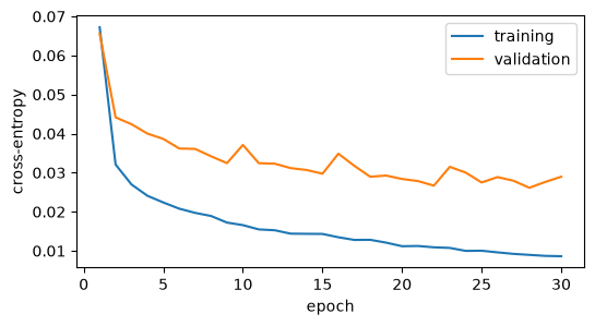
The validation loss falls with the training loss and reaches its lowest value near the end of the 30 epochs (the cell prints the epoch), so with about 21,000 records this network has not started to overfit in a way that early stopping would correct. Compare the AP of the MLP with that of logistic regression above before concluding that the extra capacity is worth its cost.

Which families does the MLP find? The test period contains c2beacon, which the model has never seen.

test_types = flows.loc[test_m, "attack_type"].to_numpy()
order = np.argsort(-logits_mlp, kind="stable")
top100 = np.zeros(len(order), bool)
top100[order[:100]] = True
mlp_family_recall = {f: float(top100[test_types == f].mean()) for f in sorted(set(test_types) - {"normal"})}
print("recall per family among the 100 highest-scored test records:", {k: round(v, 2) for k, v in mlp_family_recall.items()})

recall per family among the 100 highest-scored test records: {'bruteforce': 0.61, 'c2beacon': 0.0, 'dos': 0.7, 'exfil': 0.03, 'scan': 0.15}

3. Optimizers

The same network, from the same initial weights as the MLP above, is trained with two further optimizers for 30 epochs. The Adam run is the MLP of section 2. The learning rates are common starting points, not tuned values.

opt_specs = {
    "SGD, lr 0.1": lambda p: torch.optim.SGD(p, lr=0.1),
    "SGD with momentum 0.9, lr 0.01": lambda p: torch.optim.SGD(p, lr=0.01, momentum=0.9),
}
opt_hist = {"Adam, lr 0.001": hist_mlp}
opt_ap = {"Adam, lr 0.001": ap_mlp_last}
for name, make_opt in opt_specs.items():
    torch.manual_seed(0)
    net = make_mlp(64)                    # the same initial weights as the MLP of section 2
    h, _ = train(net, X_fit, y_fit, EPOCHS, BATCH, make_opt(net.parameters()))
    opt_hist[name] = h
    opt_ap[name] = test_ap(net)[0]
for name, h in opt_hist.items():
    print(f"{name:<32} training loss after 1 epoch {h['train'][0]:.4f}, after {EPOCHS} {h['train'][-1]:.4f}; "
          f"validation {h['val'][-1]:.4f}; test AP {opt_ap[name]:.3f}")

Adam, lr 0.001                   training loss after 1 epoch 0.0672, after 30 0.0086; validation 0.0290; test AP 0.598
SGD, lr 0.1                      training loss after 1 epoch 0.0855, after 30 0.0211; validation 0.0383; test AP 0.598
SGD with momentum 0.9, lr 0.01   training loss after 1 epoch 0.0975, after 30 0.0213; validation 0.0371; test AP 0.593

4. Weighting the loss for class imbalance

Attacks are about 2.5% of the fitting data. Setting pos_weight to the ratio of normal to attack records makes the attack records, taken together, count as much in the loss as all normal records together. This shifts the predicted probabilities upward for attacks, which changes what a fixed threshold of 0.5 does; it need not change the ranking much.

pos_weight = float((y_fit == 0).sum() / (y_fit == 1).sum())
torch.manual_seed(0)
mlp_w = make_mlp(64)
train(mlp_w, X_fit, y_fit, EPOCHS, BATCH, torch.optim.Adam(mlp_w.parameters(), lr=1e-3), pos_weight=pos_weight)
ap_weighted, logits_w = test_ap(mlp_w)
# The unweighted model is the MLP of section 2 after its last epoch.
ap_unweighted, logits_u = ap_mlp_last, logits_last

def at_half(logits):
    pred = logits > 0                     # probability above 0.5
    tp = int((pred & (y_test == 1)).sum()); fp = int((pred & (y_test == 0)).sum())
    return tp, fp, tp / max(tp + fp, 1), tp / int(y_test.sum())

tp_u, fp_u, prec_u, rec_u = at_half(logits_u)
tp_w, fp_w, prec_w, rec_w = at_half(logits_w)
print(f"pos_weight = {pos_weight:.1f}")
print(f"unweighted: AP {ap_unweighted:.3f}; at 0.5: {tp_u + fp_u} alerts, precision {prec_u:.2f}, recall {rec_u:.2f}")
print(f"weighted:   AP {ap_weighted:.3f}; at 0.5: {tp_w + fp_w} alerts, precision {prec_w:.2f}, recall {rec_w:.2f}")

pos_weight = 39.9
unweighted: AP 0.598; at 0.5: 211 alerts, precision 0.99, recall 0.48
weighted:   AP 0.604; at 0.5: 288 alerts, precision 0.83, recall 0.55

5. Overfitting and three remedies

To make overfitting visible we give a large network (two hidden layers of 256 units, about 72,000 parameters) only 600 records from the fitting period and train it full-batch for 200 epochs, so each epoch is a single iteration. Then we repeat the run with weight decay and with dropout. The validation set is the same as before.

small = rng.choice(len(X_fit), 600, replace=False)
Xs, ys = X_fit[small], y_fit[small]
print(f"small training set: {len(ys)} records, {int(ys.sum())} attacks")
BIG_EPOCHS = 200
variants = {"no regularization": {}, "weight decay 0.01": {"wd": 1e-2}, "dropout 0.5": {"dropout": 0.5}}
over = {}
for name, cfg in variants.items():
    torch.manual_seed(0)
    net = make_mlp(256, dropout=cfg.get("dropout", 0.0))
    opt = torch.optim.Adam(net.parameters(), lr=1e-3, weight_decay=cfg.get("wd", 0.0))
    h, best = train(net, Xs, ys, BIG_EPOCHS, len(Xs), opt)
    ap_last = test_ap(net)[0]
    net.load_state_dict(best[1])
    ap_best = test_ap(net)[0]
    over[name] = {"hist": h, "best_epoch": best[2], "best_val": best[0], "ap_last": ap_last, "ap_best": ap_best}
    print(f"{name:<18} final training loss {h['train'][-1]:.4f}, final validation loss {h['val'][-1]:.4f}, "
          f"lowest validation loss {best[0]:.4f} at epoch {best[2]}; test AP final {ap_last:.3f}, early-stopped {ap_best:.3f}")
n_big_params = sum(p.numel() for p in make_mlp(256).parameters())
print("parameters in the large network:", n_big_params)

fig, ax = plt.subplots(figsize=(7, 3.2))
for name, o in over.items():
    ax.plot(range(1, BIG_EPOCHS + 1), o["hist"]["val"], label=f"validation, {name}")
ax.plot(range(1, BIG_EPOCHS + 1), over["no regularization"]["hist"]["train"],
        color="k", lw=1, label="training, no regularization")
ax.set_xlabel("epoch"); ax.set_ylabel("cross-entropy"); ax.set_ylim(0, 0.25); ax.legend(fontsize=8)
plt.show()

small training set: 600 records, 19 attacks

no regularization  final training loss 0.0008, final validation loss 0.0874, lowest validation loss 0.0537 at epoch 53; test AP final 0.553, early-stopped 0.526

weight decay 0.01  final training loss 0.0278, final validation loss 0.0529, lowest validation loss 0.0529 at epoch 200; test AP final 0.517, early-stopped 0.517

dropout 0.5        final training loss 0.0040, final validation loss 0.0789, lowest validation loss 0.0554 at epoch 65; test AP final 0.544, early-stopped 0.517
parameters in the large network: 71937

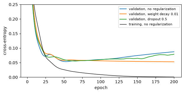
Without regularization the training loss falls toward zero while the validation loss reaches a minimum early and then rises, because the network is memorizing its 600 records. Early stopping keeps the weights from the epoch of lowest validation loss. Weight decay and dropout change the shape of the validation curve; read the printed numbers to see by how much, and notice that a lower validation loss does not always mean a higher test AP. Cross-entropy also measures how confident the scores are, while AP depends only on their order.

6. An autoencoder trained on normal traffic

The autoencoder sees the eleven numeric features of Lab 4 (no one-hot columns, no hour), standardized with statistics of the normal fitting records. It compresses each record to 3 numbers and reconstructs it; the anomaly score of a record is its squared reconstruction error. It is trained only on normal records from days 0 to 7, and its validation loss is measured on normal records from days 8 and 9.

normal_fit = fit_m & (y == 0)
normal_val = val_m & (y == 0)
sc_ae = StandardScaler().fit(numeric[normal_fit])
N_all = sc_ae.transform(numeric).astype(np.float32)
A_fit, A_val, A_test = N_all[normal_fit], N_all[normal_val], N_all[test_m]
CODE = 3

def make_ae(d=A_fit.shape[1], hidden=32, code=CODE, linear=False):
    act = nn.Identity() if linear else nn.ReLU()
    return nn.Sequential(nn.Linear(d, hidden), act, nn.Linear(hidden, code),
                         nn.Linear(code, hidden), act, nn.Linear(hidden, d))

def train_ae(net, epochs=60, seed=0):
    g = torch.Generator().manual_seed(seed)
    opt = torch.optim.Adam(net.parameters(), lr=1e-3)
    Xt, Xv = torch.from_numpy(A_fit), torch.from_numpy(A_val)
    hist = {"train": [], "val": []}
    for epoch in range(epochs):
        net.train()
        perm = torch.randperm(len(Xt), generator=g)
        for i in range(0, len(Xt), BATCH):
            b = Xt[perm[i:i + BATCH]]
            opt.zero_grad()
            loss = ((net(b) - b) ** 2).mean()
            loss.backward()
            opt.step()
        net.eval()
        with torch.no_grad():
            hist["train"].append(((net(Xt) - Xt) ** 2).mean().item())
            hist["val"].append(((net(Xv) - Xv) ** 2).mean().item())
    return hist

def recon_error(net, A):
    net.eval()
    with torch.no_grad():
        t = torch.from_numpy(A)
        return ((net(t) - t) ** 2).sum(dim=1).numpy()

torch.manual_seed(0)
ae = make_ae()
hist_ae = train_ae(ae)
score_ae = recon_error(ae, A_test)
ap_ae = average_precision_score(y_test, score_ae)
print(f"autoencoder: validation MSE per feature {hist_ae['val'][-1]:.4f}, test AP {ap_ae:.3f}")

autoencoder: validation MSE per feature 0.1034, test AP 0.366

For comparison, PCA with 3 components fitted to the same records gives a linear reconstruction, and an isolation forest is trained on the same records with the same features.

pca3 = PCA(n_components=CODE).fit(A_fit)
def pca_error(A):
    return ((A - pca3.inverse_transform(pca3.transform(A))) ** 2).sum(axis=1)
score_pca = pca_error(A_test)
ap_pca = average_precision_score(y_test, score_pca)
iso = IsolationForest(n_estimators=200, random_state=0).fit(A_fit)
score_iso = -iso.score_samples(A_test)
ap_iso = average_precision_score(y_test, score_iso)
pca_val_mse = float(pca_error(A_val).mean() / A_val.shape[1])
print(f"PCA (3 components): validation MSE per feature {pca_val_mse:.4f}, test AP {ap_pca:.3f}")
print(f"isolation forest: test AP {ap_iso:.3f}")
print(f"base rate in the test period: {y_test.mean():.3f}")

PCA (3 components): validation MSE per feature 0.3456, test AP 0.323
isolation forest: test AP 0.387
base rate in the test period: 0.041

The nonlinear autoencoder reconstructs normal validation records with a smaller error than PCA. Whether that makes it a better detector is a separate question, which the AP values answer for this data.

7. A linear autoencoder learns the principal subspace

Remove the ReLUs and the autoencoder is a composition of affine maps (each nn.Linear adds a bias), so its reconstruction is a linear map of rank at most 3 applied to the input, plus a constant vector. Baldi and Hornik (1989) showed that the minimum of the squared error is then the projection onto the subspace of the first three principal components. We train one and measure the principal angles between the subspace spanned by its decoder and the PCA subspace (0 degrees means the subspaces coincide). If the columns of \(Q_1\) and \(Q_2\) are orthonormal bases of two 3-dimensional subspaces, the cosines of their three principal angles are the singular values of \(Q_1^\top Q_2\). All three angles are 0 degrees when the subspaces coincide, and an angle of 90 degrees means that some direction of one subspace is orthogonal to the whole of the other.

torch.manual_seed(0)
lin = make_ae(linear=True)
hist_lin = train_ae(lin, epochs=40)
# The decoder maps the 3-dimensional code to the output through two linear layers (biases aside).
dec = (lin[5].weight @ lin[3].weight).detach().numpy().astype(np.float64)   # 11 x 3
q_dec, _ = np.linalg.qr(dec)
q_pca, _ = np.linalg.qr(pca3.components_.T)
cosines = np.clip(np.linalg.svd(q_dec.T @ q_pca, compute_uv=False), -1, 1)
angles = np.degrees(np.arccos(cosines))
print(f"linear autoencoder validation MSE per feature {hist_lin['val'][-1]:.4f} (PCA {pca_val_mse:.4f})")
print("principal angles between the two subspaces (degrees):", np.round(angles, 2))

linear autoencoder validation MSE per feature 0.3459 (PCA 0.3456)
principal angles between the two subspaces (degrees): [0.27 0.7  1.09]

8. Score distributions and a threshold from the alert budget

A threshold turns scores into alerts. Rather than guessing a "normal" error level, we take the alert budget of Lab 4, 25 alerts per day or 100 over the four test days, and set the threshold at the 100th highest test score. In deployment you would set it from the scores of a recent period of the same length.

BUDGET = 100
def at_budget(score):
    thr = np.sort(score)[::-1][BUDGET - 1]
    alert = score >= thr
    tp = int((alert & (y_test == 1)).sum())
    fam = {f: float(alert[test_types == f].mean()) for f in sorted(set(test_types) - {"normal"})}
    return thr, int(alert.sum()), tp / alert.sum(), tp / int(y_test.sum()), fam

thr_ae, n_alert_ae, prec_ae, rec_ae, fam_ae = at_budget(score_ae)
thr_iso, n_alert_iso, prec_iso, rec_iso, fam_iso = at_budget(score_iso)
print(f"autoencoder:      threshold {thr_ae:.3f}, {n_alert_ae} alerts, precision {prec_ae:.2f}, recall {rec_ae:.2f}")
print(f"isolation forest: threshold {thr_iso:.3f}, {n_alert_iso} alerts, precision {prec_iso:.2f}, recall {rec_iso:.2f}")
print("recall per family, autoencoder:     ", {k: round(v, 2) for k, v in fam_ae.items()})
print("recall per family, isolation forest:", {k: round(v, 2) for k, v in fam_iso.items()})

normal_above = float((score_ae[y_test == 0] >= thr_ae).mean())
attack_below = float((score_ae[y_test == 1] < thr_ae).mean())
median_normal = float(np.median(score_ae[y_test == 0]))
median_attack = float(np.median(score_ae[y_test == 1]))
print(f"share of normal test records above the threshold: {normal_above:.4f}")
print(f"share of attack test records below the threshold: {attack_below:.3f}")
print(f"median score: normal {median_normal:.3f}, attack {median_attack:.3f}")

bins = np.logspace(np.log10(max(score_ae.min(), 1e-3)), np.log10(score_ae.max()), 60)
fig, ax = plt.subplots(figsize=(7, 3.2))
ax.hist(score_ae[y_test == 0], bins=bins, alpha=0.6, density=True, label="normal")
ax.hist(score_ae[y_test == 1], bins=bins, alpha=0.6, density=True, label="attack")
ax.axvline(thr_ae, color="k", ls="--", label="threshold for 100 alerts")
ax.set_xscale("log"); ax.set_xlabel("squared reconstruction error"); ax.set_ylabel("density"); ax.legend()
plt.show()

autoencoder:      threshold 13.207, 100 alerts, precision 0.80, recall 0.19
isolation forest: threshold 0.674, 100 alerts, precision 0.76, recall 0.18
recall per family, autoencoder:      {'bruteforce': 0.43, 'c2beacon': 0.0, 'dos': 0.78, 'exfil': 0.0, 'scan': 0.06}
recall per family, isolation forest: {'bruteforce': 0.0, 'c2beacon': 0.0, 'dos': 0.44, 'exfil': 0.0, 'scan': 0.63}
share of normal test records above the threshold: 0.0020
share of attack test records below the threshold: 0.815
median score: normal 0.723, attack 2.406

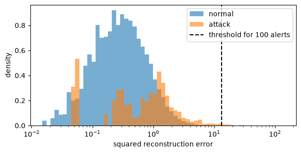
The two distributions overlap heavily. Most attacks fall below the threshold and are not reported, and the alerts above it include normal records. Lesson 5.3 discusses why. Reconstruction error measures how unusual a record is relative to the normal training data, and several attack families, exfil and c2beacon in particular, are not unusual in that sense (the autoencoder flags none of their records within the budget).

Try this

Change CODE to 2 and to 6. Predict whether the validation MSE and the test AP move in the same direction, then run it.
Train the MLP for 100 epochs instead of 30. At which epoch does the validation loss stop improving?
Replace weight_decay in Adam by torch.optim.AdamW with the same value. The two are not the same algorithm; compare their validation curves.
Train the autoencoder on all records of days 0 to 7, attacks included, and measure the change in AP.

Results summary

results = {
    "n_fit": int(len(y_fit)), "n_fit_attacks": int(y_fit.sum()),
    "n_val": int(len(y_val)), "n_val_attacks": int(y_val.sum()),
    "n_test": int(len(y_test)), "n_test_attacks": int(y_test.sum()),
    "n_features": int(X.shape[1]),
    "batch": BATCH, "iters_per_epoch": iters_per_epoch, "epochs": EPOCHS,
    "ap_logreg": float(ap_logreg), "ap_mlp_last": float(ap_mlp_last), "ap_mlp_best": float(ap_mlp_best),
    "mlp_best_epoch": int(best_mlp[2]), "mlp_best_val": float(best_mlp[0]),
    "mlp_final_train": float(hist_mlp["train"][-1]), "mlp_final_val": float(hist_mlp["val"][-1]),
    "mlp_recall_c2beacon_top100": mlp_family_recall["c2beacon"],
    "pos_weight": pos_weight,
    "ap_unweighted": float(ap_unweighted), "ap_weighted": float(ap_weighted),
    "alerts_half_unweighted": tp_u + fp_u, "prec_half_unweighted": prec_u, "rec_half_unweighted": rec_u,
    "alerts_half_weighted": tp_w + fp_w, "prec_half_weighted": prec_w, "rec_half_weighted": rec_w,
    "small_n": int(len(ys)), "small_attacks": int(ys.sum()), "big_epochs": BIG_EPOCHS, "big_params": int(n_big_params),
    "ae_code": CODE, "ap_ae": float(ap_ae), "ap_pca": float(ap_pca), "ap_iso": float(ap_iso),
    "ae_val_mse": float(hist_ae["val"][-1]), "pca_val_mse": pca_val_mse, "lin_val_mse": float(hist_lin["val"][-1]),
    "max_angle_deg": float(angles.max()),
    "budget": BUDGET, "thr_ae": float(thr_ae), "prec_ae_budget": float(prec_ae), "rec_ae_budget": float(rec_ae),
    "prec_iso_budget": float(prec_iso), "rec_iso_budget": float(rec_iso),
    "fa_ae_budget": int(round(n_alert_ae * (1 - prec_ae))), "tp_ae_budget": int(round(n_alert_ae * prec_ae)),
    "ae_normal_above": normal_above, "ae_attack_below": attack_below,
    "ae_median_normal": median_normal, "ae_median_attack": median_attack,
    "test_base_rate": float(y_test.mean()),
}
for name, o in over.items():
    key = {"no regularization": "none", "weight decay 0.01": "wd", "dropout 0.5": "drop"}[name]
    results[f"over_{key}_final_train"] = float(o["hist"]["train"][-1])
    results[f"over_{key}_final_val"] = float(o["hist"]["val"][-1])
    results[f"over_{key}_best_val"] = float(o["best_val"])
    results[f"over_{key}_best_epoch"] = int(o["best_epoch"])
    results[f"over_{key}_ap_last"] = float(o["ap_last"])
    results[f"over_{key}_ap_best"] = float(o["ap_best"])
for name, h in opt_hist.items():
    key = {"SGD, lr 0.1": "sgd", "SGD with momentum 0.9, lr 0.01": "mom", "Adam, lr 0.001": "adam"}[name]
    results[f"opt_{key}_train1"] = float(h["train"][0])
    results[f"opt_{key}_train_last"] = float(h["train"][-1])
    results[f"opt_{key}_val_last"] = float(h["val"][-1])
    results[f"opt_{key}_ap"] = float(opt_ap[name])
for f, v in fam_ae.items():
    results[f"recall_{f}_ae"] = v
    results[f"recall_{f}_iso"] = fam_iso[f]
for k, v in results.items():
    print(f"{k:<28} {v}")

hist_bins = np.logspace(-3, np.log10(float(score_ae.max())) + 0.01, 61)
export = {
    "mlp_hist": hist_mlp,
    "opt_hist": {k: v["train"] for k, v in opt_hist.items()},
    "over_hist": {k: o["hist"] for k, o in over.items()},
    "over_best_epoch": {k: o["best_epoch"] for k, o in over.items()},
    "ae_hist": hist_ae,
    "hist_bins": hist_bins.tolist(),
    "hist_normal": np.histogram(np.clip(score_ae[y_test == 0], 1e-3, None), bins=hist_bins)[0].tolist(),
    "hist_attack": np.histogram(np.clip(score_ae[y_test == 1], 1e-3, None), bins=hist_bins)[0].tolist(),
    "thr_ae": float(thr_ae),
    "family_recall": {"autoencoder": fam_ae, "isolation forest": fam_iso},
    "ap": {"logistic regression": float(ap_logreg), "MLP": float(ap_mlp_best), "autoencoder": float(ap_ae),
           "PCA": float(ap_pca), "isolation forest": float(ap_iso)},
}

# When the course build runs this notebook, it saves the numbers for the lesson pages.
if os.environ.get("COURSE_RESULTS"):
    import json
    with open(os.environ["COURSE_RESULTS"], "w") as f:
        json.dump({"results": results, "data": export}, f)

n_fit                        21056
n_fit_attacks                515
n_val                        5219
n_val_attacks                93
n_test                       10495
n_test_attacks               432
n_features                   22
batch                        256
iters_per_epoch              83
epochs                       30
ap_logreg                    0.5434462071675478
ap_mlp_last                  0.5976297353956468
ap_mlp_best                  0.5978310954781999
mlp_best_epoch               28
mlp_best_val                 0.026138080283999443
mlp_final_train              0.008622653782367706
mlp_final_val                0.028961408883333206
mlp_recall_c2beacon_top100   0.0
pos_weight                   39.88543689320388
ap_unweighted                0.5976297353956468
ap_weighted                  0.6038702496904084
alerts_half_unweighted       211
prec_half_unweighted         0.985781990521327
rec_half_unweighted          0.48148148148148145
alerts_half_weighted         288
prec_half_weighted           0.8298611111111112
rec_half_weighted            0.5532407407407407
small_n                      600
small_attacks                19
big_epochs                   200
big_params                   71937
ae_code                      3
ap_ae                        0.36551241911694066
ap_pca                       0.32253028053418814
ap_iso                       0.38722397513842555
ae_val_mse                   0.10337096452713013
pca_val_mse                  0.3455526828765869
lin_val_mse                  0.34585705399513245
max_angle_deg                1.0865131949123545
budget                       100
thr_ae                       13.207266807556152
prec_ae_budget               0.8
rec_ae_budget                0.18518518518518517
prec_iso_budget              0.76
rec_iso_budget               0.17592592592592593
fa_ae_budget                 20
tp_ae_budget                 80
ae_normal_above              0.0019874788830368676
ae_attack_below              0.8148148148148148
ae_median_normal             0.7227367162704468
ae_median_attack             2.4058313369750977
test_base_rate               0.041162457317113876
over_none_final_train        0.0007551372400484979
over_none_final_val          0.0873948484659195
over_none_best_val           0.053686920553445816
over_none_best_epoch         53
over_none_ap_last            0.5533140871529789
over_none_ap_best            0.5256943990145175
over_wd_final_train          0.027810946106910706
over_wd_final_val            0.05294163525104523
over_wd_best_val             0.05294163525104523
over_wd_best_epoch           200
over_wd_ap_last              0.5167517119286146
over_wd_ap_best              0.5167517119286146
over_drop_final_train        0.00403786962851882
over_drop_final_val          0.07886990159749985
over_drop_best_val           0.055442050099372864
over_drop_best_epoch         65
over_drop_ap_last            0.5441171956070022
over_drop_ap_best            0.5166638406648982
opt_adam_train1              0.06720653921365738
opt_adam_train_last          0.008622653782367706
opt_adam_val_last            0.028961408883333206
opt_adam_ap                  0.5976297353956468
opt_sgd_train1               0.08551156520843506
opt_sgd_train_last           0.021091409027576447
opt_sgd_val_last             0.03827210143208504
opt_sgd_ap                   0.598371454677
opt_mom_train1               0.09754718095064163
opt_mom_train_last           0.021289143711328506
opt_mom_val_last             0.037133969366550446
opt_mom_ap                   0.5926470295073878
recall_bruteforce_ae         0.43373493975903615
recall_bruteforce_iso        0.0
recall_c2beacon_ae           0.0
recall_c2beacon_iso          0.0
recall_dos_ae                0.78
recall_dos_iso               0.44
recall_exfil_ae              0.0
recall_exfil_iso             0.0
recall_scan_ae               0.05813953488372093
recall_scan_iso              0.627906976744186