Unit 5 · Lesson 5.1
Neurons, layers and backpropagation
Logistic regression (Lesson 3.1) draws one linear boundary through feature space. Many security problems need more, such as a combination of features that matters only when both are high, a pattern in a byte sequence, or an interaction between time of day and destination. A neural network builds such functions by composing simple units, and it is trained by the same gradient descent as logistic regression. What makes training possible at scale is an efficient way to compute the gradient of the loss with respect to every weight, the algorithm called backpropagation. This lesson defines the neuron and the multilayer perceptron, explains why nonlinear activations are necessary, states what the universal approximation theorem does and does not promise, and then works through backpropagation on a network small enough to check by hand. The same gradient computation reappears in Unit 7, where an attacker uses it to find inputs that fool a model.
The neuron and its activation
A neuron (or unit) receives inputs \(x \in \mathbb{R}^d\), computes a weighted sum plus a bias, the pre-activation \(z = w^\top x + b\), and outputs \(g(z)\) for some fixed activation function \(g\). Logistic regression is a single neuron with the sigmoid activation \(\sigma(z) = 1/(1 + e^{-z})\). Three activations are common, shown with their derivatives in Figure 5.1:
- the sigmoid \(\sigma(z)\), with derivative \(\sigma(z)(1 - \sigma(z))\), which is at most 0.25;
- the hyperbolic tangent \(\tanh(z)\), with derivative \(1 - \tanh^2(z)\), which is at most 1;
- the rectified linear unit \(\mathrm{ReLU}(z) = \max(0, z)\), with derivative 0 for \(z < 0\) and 1 for \(z > 0\).
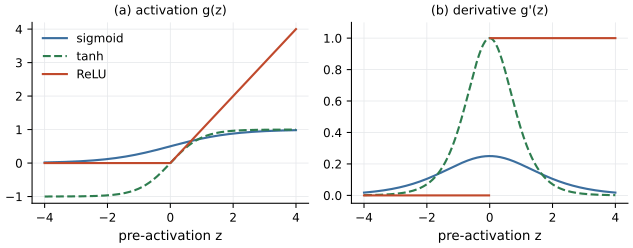
Figure 5.1. (a) Three activation functions g(z) as functions of the pre-activation z, namely the sigmoid, the hyperbolic tangent and the rectified linear unit (ReLU). (b) Their derivatives. The sigmoid and tanh derivatives fall toward zero for large |z| (saturation); the ReLU derivative is 0 for negative z and 1 for positive z, and is undefined at z = 0, where software uses 0.
ReLU is piecewise linear, two linear pieces joined at zero, and a network built from ReLUs computes a piecewise linear function of its input. The sigmoid and tanh saturate. For large \(|z|\) their derivatives are nearly zero, so gradients passing through many saturated units shrink. ReLU does not saturate for positive inputs, and Goodfellow et al. (2016) call it the default recommendation for the hidden units of modern neural networks. Its weakness is the other piece. A unit whose pre-activation is negative for every training record passes no gradient at all and stops learning, a so-called dead unit.
Why the activation must be nonlinear
Stack two layers without an activation between them. The first computes \(W^{(1)} x + b^{(1)}\) and the second \(W^{(2)} (W^{(1)} x + b^{(1)}) + b^{(2)}\), which simplifies to
a single affine map \(x \mapsto A x + c\) with \(A = W^{(2)} W^{(1)}\) and \(c = W^{(2)} b^{(1)} + b^{(2)}\). The same holds for any number of layers. Without nonlinear activations, a deep network can represent nothing that one affine layer cannot, and a stack of such layers followed by a sigmoid output is exactly logistic regression. Note that the result is affine, not linear (it has an offset), and its graph is a straight line only when the input is one-dimensional. A nonlinearity between the layers, even one as simple as ReLU, breaks the collapse.
Show the answer
The hidden layer has \(10 \times 50 + 50 = 550\) parameters and the output unit \(50 + 1 = 51\), for 601 in total. By equation \eqref{eq:affine}, the composition of the hidden layer and the output's pre-activation is a single affine map from 10 inputs to one number, so the network computes \(\sigma(A x + c)\) for some \(1 \times 10\) matrix \(A\) and \(c \in \mathbb{R}\), which is logistic regression with 11 parameters. The extra 590 parameters add no expressive power, only redundancy.
The multilayer perceptron
A multilayer perceptron (MLP) applies layers in sequence. With \(h^{(0)} = x\), each hidden layer \(l = 1, \dots, L-1\) computes
where \(W^{(l)}\) is a matrix with one row per unit of layer \(l\) and one column per unit of layer \(l-1\), \(b^{(l)}\) is a vector of biases and \(g\) is applied elementwise. For binary detection the output layer is a single unit with pre-activation \(a = w^{(L)\top} h^{(L-1)} + b^{(L)}\), often called the logit, and predicted probability \(p = \sigma(a)\). The loss for one record with label \(y \in \{0, 1\}\) is the binary cross-entropy of Lesson 3.1,
and the training loss is its average over the training records. Differentiating \eqref{eq:bce} with respect to the logit gives a simple result. Since \(\partial \ell/\partial p = -y/p + (1-y)/(1-p)\) and \(\partial p/\partial a = p(1 - p)\),
the prediction error. Frameworks also provide the sigmoid and the cross-entropy as one combined operation that takes the logit as input (in PyTorch, BCEWithLogitsLoss), because it is numerically safer than computing \(p\) first and taking its logarithm.
What one hidden layer can represent
Cybenko (1989) proved that for any continuous sigmoidal function \(\varphi\), meaning one that tends to 1 as its argument tends to \(+\infty\) and to 0 as it tends to \(-\infty\), finite sums of the form \(G(x) = \sum_{j=1}^{N} \alpha_j \varphi(w_j^\top x + b_j)\) are dense in the continuous functions on the unit cube \([0, 1]^d\). For every continuous \(f\) on the cube and every \(\varepsilon > 0\) there is such a sum with \(|G(x) - f(x)| < \varepsilon\) at every point of the cube. Such a sum is a network with one hidden layer of \(N\) units with activation \(\varphi\) and a linear output. Hornik et al. (1989) proved, more generally, that networks with as few as one hidden layer and arbitrary squashing activation functions can approximate any Borel measurable function from one finite-dimensional space to another to any desired degree of accuracy, provided sufficiently many hidden units are available. As Goodfellow et al. (2016) summarize, later results extended such theorems to a wider class of activations that includes ReLU.
These are existence results, and their limits are part of the statement. They do not say how many hidden units are needed, which may be impractically many; Hornik et al. state explicitly that their results do not address that question. They do not say that gradient descent will find the approximating weights, nor that weights fitted to a finite training set will generalize. Goodfellow et al. separate the two failures, an optimization algorithm that cannot find the right parameters and a training algorithm that chooses the wrong function because of overfitting. For a detector, the theorem settles only whether a large enough network can represent a good decision function. Whether a trained network detects attacks depends on the data, labels, features and evaluation, which the theorem does not address.
Backpropagation computes gradients
Training an MLP by gradient descent requires \(\partial \mathcal{L}/\partial \theta\) for every parameter \(\theta\), where \(\mathcal{L}\) is the training loss. The chain rule gives each of these derivatives, and backpropagation organizes the computation so that its cost is of the same order as that of the forward computation (Goodfellow et al., 2016). It runs in two passes. The forward pass computes and stores every pre-activation and activation, layer by layer. The backward pass starts from \(\partial \ell/\partial a\) at the output and moves toward the input, computing at each layer the derivative of the loss with respect to that layer's pre-activations from the one already computed for the layer above. For a hidden layer \(l\), writing \(\delta^{(l)} = \partial \ell/\partial z^{(l)}\) for the vector of derivatives with respect to its pre-activations \(z^{(l)} = W^{(l)} h^{(l-1)} + b^{(l)}\),
for \(l = L-1, \dots, 1\). The recursion starts at the output, where \(z^{(L)} = a\), \(W^{(L)} = w^{(L)\top}\) (the output weights as a one-row matrix) and \(\delta^{(L)} = p - y\) by \eqref{eq:dlda}. The gradients of each layer's own parameters follow directly,
where \(\odot\) is the elementwise product. Each layer reuses the quantity computed for the layer above instead of recomputing the chain from the output, which is what makes the method efficient.
Rumelhart et al. (1986) described this procedure for layered networks of sigmoid units and showed that hidden units trained this way come to represent important features of the task. Their paper computes the derivatives in a backward pass (their equations 4 to 7) and then, as a separate step, changes each weight in proportion to the accumulated derivative, \(\Delta w = -\eta\, \partial E/\partial w\) (their equation 8, where \(E\) is their total error, half the sum of squared output errors over the training cases, and the step size \(\eta\) is written \(\varepsilon\)), optionally with a momentum term. The paper uses "back-propagation" for the whole learning procedure. Modern usage is narrower. Goodfellow et al. point out that the term is often misunderstood as the whole learning algorithm, whereas it refers only to the method for computing the gradient, while another algorithm, such as stochastic gradient descent, uses that gradient to perform learning. This course follows the modern usage. Backpropagation produces gradients and changes no weight; the optimizer (Lesson 5.2) applies the update.
A worked example: one step for a 2-2-1 network
Figure 5.2 shows a network with two inputs, two hidden ReLU units and one sigmoid output. Its parameters are the hidden weights \(W\) (row \(j\) holds the weights into hidden unit \(j\)), hidden biases \(b\), output weights \(v\) and output bias \(c\),
One training record has input \(x = (1, 2)\) and label \(y = 1\), an attack.
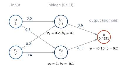
Figure 5.2. The 2-2-1 network of the worked example. Arrows carry the weights of equation \eqref{eq:params}; each node shows its value in the forward pass for the input x = (1, 2). Below the hidden units are their pre-activations z and biases b, and below the output unit its logit a and bias c. The output p is the predicted probability of attack.
Forward pass. The hidden pre-activations are \(z_1 = 0.5 \cdot 1 - 0.2 \cdot 2 + 0.1 = 0.2\) and \(z_2 = 0.3 \cdot 1 + 0.4 \cdot 2 - 0.1 = 1.0\). Both are positive, so \(h = (0.2, 1.0)\). The logit is \(a = 0.6 \cdot 0.2 - 0.5 \cdot 1.0 + 0.2\), which equals \(-0.18\), the probability is \(p = \sigma(-0.18) \approx 0.4551\), and the loss is \(\ell = -\ln 0.4551 \approx 0.7872\). The network leans toward "normal" for a record that is an attack.
Backward pass. By \eqref{eq:dlda}, \(\partial \ell/\partial a = p - y \approx -0.5449\). The logit is \(a = v^\top h + c\), so
and \(\partial \ell/\partial c = p - y \approx -0.5449\).
The gradient flows on to the hidden activations through the output weights, \(\partial \ell/\partial h = (p - y)\, v\), which is approximately \((-0.3269, 0.2724)\).
ReLU passes the gradient unchanged where \(z > 0\), which holds for both units, so \(\partial \ell/\partial z = (-0.3269, 0.2724)\). Since \(z_j = \sum_i W_{ji} x_i + b_j\), the derivative with respect to \(W_{ji}\) is \(\partial \ell/\partial z_j \cdot x_i\),
The signs can be read off the network. Raising the output probability requires a larger logit. The first hidden unit feeds the output through the positive weight 0.6, and both inputs are positive, so increasing its incoming weights helps and their gradient is negative; the second feeds it through \(-0.5\), so its incoming weights should decrease and their gradient is positive.
The update is a separate step. Plain gradient descent with learning rate \(\eta = 0.5\) subtracts \(0.5\) times each gradient, giving
With the new parameters the same record gives \(p \approx 0.7692\) and \(\ell \approx 0.2624\). One step on one record has moved the prediction strongly toward the label. On a full training set the gradients of different records pull in different directions, and full-batch gradient descent follows their average, the gradient of the mean loss, so no single record moves the parameters this far. The next section trains a network in this way with the same learning rate of 0.5.
Lab 5a computes these numbers in NumPy and checks them twice. Central finite differences, \([\ell(\theta + \epsilon) - \ell(\theta - \epsilon)]/(2\epsilon)\) with \(\epsilon = 10^{-6}\), agree with every analytic gradient to within 1.3e-10, and PyTorch's automatic differentiation (autograd), which runs the backward pass of equation \eqref{eq:backprop} over the recorded operations, reproduces them (the largest absolute difference is 0 in double precision). Gradient checking of this kind is a standard test of a hand-written backward pass.
Show the answer
Then \(z_1 = 0.5 - 0.4 - 0.6 = -0.5 < 0\), so \(h_1 = 0\) and the ReLU derivative at \(z_1\) is 0. The gradients with respect to \(W_{11}\), \(W_{12}\) and \(b_1\) are all zero, because \(\partial \ell/\partial z_1 = 0\), and so is \(\partial \ell/\partial v_1 = (p - y) h_1 = 0\). The second unit still learns. Its pre-activation \(z_2 = 1.0\) is still positive, so its weights, bias and output weight receive nonzero gradients (with slightly different values, because \(p\) has changed to about 0.4256). If the first unit's pre-activation were negative for every training record, it would never receive a gradient, which is the dead-unit problem.
From one record to a decision boundary
A single step on one record shows the mechanics. Training repeats it over many records. In Lab 5a, a network with 2 inputs, 16 ReLU hidden units and a sigmoid output is trained by full-batch gradient descent on 400 points of an XOR-like problem, where points in the first and third quadrants are one class and points in the second and fourth the other, with a small share of labels flipped. No single line separates these classes, and logistic regression, which can only draw a line, does little better than chance on them. Figure 5.3 shows the boundary during training. The loss falls from 0.679 to 0.322 in 600 steps, and the training accuracy rises from 0.60 to 0.93. It stays below 1 because 5.5% of the labels were flipped. Even the exact quadrant rule misclassifies those points and so scores one minus that share, slightly above the network's final accuracy; going beyond the rule would mean fitting the flipped labels.
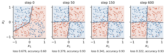
Figure 5.3. Decision boundary (dark line, predicted probability 0.5) of a 2-16-1 ReLU network trained by full-batch gradient descent with learning rate 0.5 on 400 synthetic points of an XOR-like problem (Lab 5a), at steps 0, 50, 150 and 600. Red points are class 1, blue points class 0; shading shows the predicted class. Below each panel are the mean cross-entropy and the training accuracy at that step.
The boundary is made of straight segments, as expected, because the logit of a ReLU network is a piecewise linear function of the input and the boundary is the set where the logit is zero. It starts wherever the random initialization put it and bends into the quadrant structure within the first few dozen steps. After that the training accuracy barely changes, as the labels under the panels show, while the loss keeps falling as the predicted probabilities become more confident.
Security notes
Two points matter beyond the mechanics. First, the network's capacity to fit arbitrary functions includes the capacity to fit artifacts of the training data, such as the identity of a sensor or a leaked column like ticket_opened, and the theorem of the previous sections offers no protection against learning the wrong function. Second, the backward pass can continue one step further, from the first layer to the input, giving \(\partial \ell/\partial x\). That gradient tells an attacker how to change an input to change the output, and it is the basis of the gradient attacks of Unit 7.
What the lab shows
Lab 5a
Backpropagation by hand, then in PyTorch
Open in ColabRead with outputsNotebook on GitHubAbout 1 minute to run on a laptop CPU
Lab 5a implements the forward and backward passes of the 2-2-1 network, checks every gradient against finite differences and PyTorch autograd, applies one update, and then trains the larger network on the XOR-like data while recording the decision boundary.
Summary
A neuron applies an activation function to an affine combination of its inputs, and a multilayer perceptron composes layers of neurons. Without nonlinear activations any stack of layers collapses into a single affine map, so the nonlinearity, often the piecewise linear ReLU, is what gives depth its power. Cybenko and Hornik et al. showed that one hidden layer with enough units can approximate continuous or measurable functions arbitrarily well, but not how many units are needed or that training will find them. Backpropagation applies the chain rule backward through the network to compute the gradient of the loss with respect to every parameter, at a cost comparable to the forward pass; for a sigmoid output with cross-entropy loss the backward pass starts from \(p - y\). The weights change only when an optimizer uses those gradients, and the worked 2-2-1 example, checked by finite differences and autograd, shows each step of that process.
References
- Cybenko, G. (1989). Approximation by superpositions of a sigmoidal function. Mathematics of Control, Signals, and Systems, 2(4), 303-314. https://doi.org/10.1007/BF02551274
- Goodfellow, I., Bengio, Y., and Courville, A. (2016). Deep Learning. MIT Press. https://www.deeplearningbook.org
- Hornik, K., Stinchcombe, M., and White, H. (1989). Multilayer feedforward networks are universal approximators. Neural Networks, 2(5), 359-366. https://doi.org/10.1016/0893-6080(89)90020-8
- Rumelhart, D. E., Hinton, G. E., and Williams, R. J. (1986). Learning representations by back-propagating errors. Nature, 323(6088), 533-536. https://doi.org/10.1038/323533a0