Unit 4 · Lesson 4.2
Principal component analysis
Security data has many features, and many of them move together. Bytes sent, packets sent and connection duration rise and fall together; a host that opens many connections also tends to contact many destinations. Principal component analysis (PCA) replaces correlated features by a smaller number of uncorrelated combinations that keep as much of the variation as possible. It is used to draw high-dimensional data in two dimensions, to compress features before another model, and, through the part of a record that the main combinations cannot explain, to score anomalies. This lesson derives PCA from the covariance matrix and from the singular value decomposition, works a two-dimensional example exactly, and then turns to the use of PCA residuals for detecting network-wide traffic anomalies and to the limits of that approach.
Directions of maximum variance
Let \(x_1, \dots, x_n \in \mathbb{R}^p\) be the records and \(\bar{x}\) their mean. Stack the centered records \(x_i - \bar{x}\) as the rows of an \(n \times p\) matrix \(X\). The sample covariance matrix is
a symmetric \(p \times p\) matrix whose diagonal holds the variances of the features and whose off-diagonal entries hold their covariances. For a unit vector \(a \in \mathbb{R}^p\), the projections \(X a\) are the coordinates of the records along the direction \(a\), and their variance is \(a^\top S a\).
The first principal component is the direction that maximizes this variance. Maximizing \(a^\top S a\) subject to \(a^\top a = 1\) with a Lagrange multiplier \(\lambda\) gives the condition \(S a = \lambda a\), so \(a\) must be an eigenvector of \(S\), and the variance along it, \(a^\top S a = \lambda\), is the corresponding eigenvalue (Jolliffe and Cadima, 2016). The maximum is attained by the eigenvector with the largest eigenvalue. The second component maximizes variance among directions orthogonal to the first, and so on. Writing the eigenvalues in decreasing order \(\lambda_1 \ge \lambda_2 \ge \dots \ge \lambda_p \ge 0\) with orthonormal eigenvectors \(a_1, \dots, a_p\),
The vectors \(a_j\) are the loadings and the projections \(X a_j\) are the scores of the \(j\)-th principal component. The scores of different components are uncorrelated. The signs of the eigenvectors are arbitrary, so the same analysis run with different software or on slightly different data may flip a component, which is harmless but worth knowing before comparing plots.
Pearson (1901) arrived at the same directions from the opposite side. He asked for the line or plane of closest fit to a cloud of points, in the sense of the smallest sum of squared perpendicular distances, and showed that the best-fitting plane passes through the centroid of the points and depends only on their means, variances and covariances. Minimizing the squared distance to a \(q\)-dimensional subspace through the mean and maximizing the variance of the projections onto it are the same problem, because for every record the squared distance to the mean splits into the squared length of the projection plus the squared length of the residual. That identity is what makes the residual useful for anomaly detection later in this lesson.
The same components from the singular value decomposition
Any \(n \times p\) matrix of rank \(r\) can be written as \(X = U L A^\top\), where \(U\) (\(n \times r\)) and \(A\) (\(p \times r\)) have orthonormal columns and \(L\) is diagonal with the positive singular values \(l_1 \ge \dots \ge l_r\). Substituting into \eqref{eq:cov} gives \((n-1) S = A L^2 A^\top\), so the columns of \(A\), the right singular vectors of \(X\), are the eigenvectors of \(S\), the eigenvalues are \(\lambda_j = l_j^2/(n-1)\), and the scores are the columns of \(U L\) (Jolliffe and Cadima, 2016). Both routes give the same components, and scikit-learn's PCA chooses between them according to the shape of the data. It centers the data with the mean of the data it is fitted on and stores the loadings as the rows of components_ and the eigenvalues as explained_variance_.
How many components to keep
The total variance is the sum of the feature variances, the trace of \(S\), which equals \(\sum_j \lambda_j\). The share of the total explained by the first \(q\) components is
A common rule keeps the smallest \(q\) for which \(\rho_q\) reaches a chosen level. Jolliffe and Cadima (2016) describe 70% as a common, if subjective, cut-off, and note that plots often use the first two or three components whatever share they explain. Whichever level you choose, apply it as stated. If the rule is 90%, you keep the smallest number of components whose cumulative share is at least 0.90, no more and no fewer, and you report the share actually reached.
A worked example in two dimensions
Take five records with two features, (1, 2), (2, 1), (3, 4), (4, 3) and (5, 5). Their mean is (3, 3), and the centered records are (−2, −1), (−1, −2), (0, 1), (1, 0) and (2, 2). The sums of squares and cross-products of the centered records are \(\sum_i X_{i1}^2 = 10\), \(\sum_i X_{i2}^2 = 10\) and \(\sum_i X_{i1} X_{i2} = 8\), so with \(n - 1 = 4\),
The eigenvalues solve \((2.5 - \lambda)^2 - 4 = 0\), which gives \(\lambda_1 = 4.5\) and \(\lambda_2 = 0.5\). The eigenvectors are \(a_1 = (1, 1)/\sqrt{2}\) and \(a_2 = (1, -1)/\sqrt{2}\). Their inner product is \((1 - 1)/2 = 0\), so they are orthogonal, and both principal axes pass through the mean (3, 3), as Figure 4.4 shows. The total variance is \(2.5 + 2.5 = 5 = 4.5 + 0.5\), and the first component explains \(\rho_1 = 4.5/5 = 0.90\). Under a 90% rule, one component is kept, because one already reaches 90%.
The scores on the first component are the centered records multiplied by \(a_1\), namely \((-3, -3, 1, 1, 4)/\sqrt{2}\), whose squares sum to \(36/2 = 18\), so their variance is \(18/4 = 4.5 = \lambda_1\). The scores on the second component are \((-1, 1, -1, 1, 0)/\sqrt{2}\), with variance 0.5. Keeping one component reconstructs each record as its projection onto the first axis, and the squared residual is the squared second score, 0.5 for each of the first four records and 0 for (5, 5), which lies exactly on the axis. The squared residuals add up to \(2 = (n-1)\lambda_2\), the sum of squares that the dropped component carried. The singular values of the centered data are \(\sqrt{4 \times 4.5} = \sqrt{18} \approx 4.24\) and \(\sqrt{4 \times 0.5} = \sqrt{2} \approx 1.41\), consistent with \(\lambda_j = l_j^2/(n-1)\).
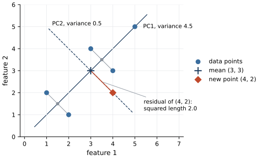
Figure 4.4. The worked example of this lesson, with five points (blue), their mean (3, 3) (cross), the first principal axis (solid, variance 4.5) and the second (dashed, variance 0.5), both through the mean and orthogonal to each other. Gray segments join each point to its projection on the first axis. A new point (4, 2) (red diamond) projects onto the mean; its residual, the red segment, has squared length 2.0, four times the largest squared residual among the original points (0.5).
Now score a new record (4, 2). Centered, it is (1, −1). Its first score is \((1 - 1)/\sqrt{2} = 0\) and its second is \((1 + 1)/\sqrt{2} = \sqrt{2}\), so its squared residual is 2. The record is not far from the mean, at distance \(\sqrt{2}\), and each of its features is within the range of the data. What is unusual is the combination. In no training record did the two features deviate from their means in opposite directions, and in this one they do. The residual measures exactly that departure from the correlation structure, which a check on each feature separately would miss.
Show the answer
It would fall. The record (1, 5) lies far from the mean along the direction (−1, 1), which is the second principal axis of the original data. Its offset from the original mean, (−2, 2), has no component along (1, 1). Adding it therefore raises the variance along (−1, 1), from 0.5 to about 1.73, while the variance along (1, 1) falls from 4.5 to 3.6, because the sum of squares in that direction is unchanged and \(n - 1\) grows. Hence \(\lambda_2\) grows relative to \(\lambda_1\), and the first component's share drops from 0.90 to 0.675. This is also how anomalies in the training data contaminate PCA. A few extreme records can pull a principal axis toward themselves, after which they no longer have large residuals.
Standardize before PCA
PCA maximizes variance, and variance depends on units. If one feature is a byte count in the millions and another a rate between 0 and 1, the first component will be almost exactly the byte count, because its variance dwarfs everything else, and changing bytes to kilobytes would change the answer. Jolliffe and Cadima (2016) explain that PCA on standardized features, each centered and divided by its standard deviation, is the same as PCA of the correlation matrix, is invariant to linear changes of units, and is the appropriate choice when the scale of each feature could change independently of the others. Heavy-tailed counts need one more step. A log transform first, as in Lesson 2.1, keeps a few enormous transfers from defining the leading components on their own.
The scaling statistics and the components themselves are learned from data, so both are fitted on the training period and applied unchanged to later data, as with any learned preprocessing step (Lesson 2.2).
PCA on the course data
Lab 4 applies PCA to eleven flow features of the training period, seven of them log-transformed and all eleven standardized. Figure 4.5 shows the explained variance. The first component explains 34.0% of the total and the second 18.8%, so a two-dimensional picture shows 52.8% of it. Under a 90% rule the lab keeps 7 components, which together explain 92.2%; one component fewer would explain 87.9%, short of the threshold.
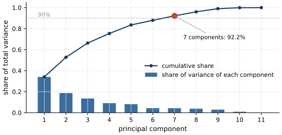
Figure 4.5. Explained variance of the eleven principal components of the standardized training features in Lab 4 (days 0 to 9). Bars give the share of the total variance of each component, the line the cumulative share, equation \eqref{eq:evr}. The dotted line marks 90%, and the red point the smallest number of components whose cumulative share reaches it.
Figure 4.6 plots a sample of training records on the first two components. Panel (a) colors them by label, which PCA never saw. Some attack groups sit at the edges of the cloud, but other attacks lie inside the dense regions occupied by normal traffic, and the dense regions themselves correspond to kinds of traffic, not to classes. Panel (b) shows the DBSCAN clusters of Lesson 4.1 on the same projection. Most noise points lie on the sparse fringe where many attacks also lie, which is why density and distance carry some signal about attacks, and the fringe also contains normal records.
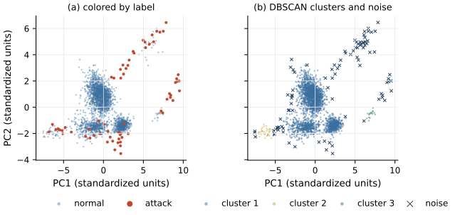
Figure 4.6. A random sample of 3,000 training records of Lab 4 projected on the first two principal components (standardized units), which together explain 52.8% of the variance. (a) Colored by label (normal blue, attack red). The label was not used to compute the projection. (b) The same points colored by DBSCAN cluster (eps and min_samples as in Lab 4); dark crosses are points labeled noise.
Reconstruction error as an anomaly score
Let \(P\) be the \(p \times q\) matrix whose columns are the first \(q\) loadings. The reconstruction of a record \(x\) from \(q\) components is \(\hat{x} = \bar{x} + P P^\top (x - \bar{x})\), and its reconstruction error is
the squared length of the part of \(x\) that the leading components do not explain, the red segment in Figure 4.4. A record that follows the correlations of the training data has a small error even when it is far from the mean along a leading axis. A record that breaks them has a large error. Jolliffe and Cadima mention outlier detection as one of the situations in which the last components, not the first, are of interest.
Lakhina et al. (2004) used this idea on the traffic of entire networks. Each record was the vector of traffic volumes on all links of a backbone network in a ten-minute interval, and they observed that although each network had more than 40 links, 3 or 4 principal components captured most of the variance of the link time series. They placed the leading components (four in each of their datasets) in a normal subspace and the rest in an anomalous subspace, computed the squared prediction error, which is \eqref{eq:recon}, for each interval, and raised an alarm when it exceeded a threshold derived from a statistical test, the Q-statistic. On data from the Sprint-Europe and Abilene backbones the method consistently detected the largest volume anomalies with a very low false alarm rate and identified the origin-destination flow responsible.
Follow-up work found the method harder to operate than this suggests. Ringberg et al. (2007) analyzed a week of traffic from the Abilene and Geant backbones and found that the false positive rate was very sensitive to small differences in the number of components placed in the normal subspace, that effectiveness depended on how traffic was aggregated, that a large anomaly could pollute the normal subspace, and that identifying the flow responsible was inherently difficult. The first and third problems carry over to any use of PCA for detection. The number of components is a tuning parameter that changes the alarms, and training data containing attacks shapes the subspace that is supposed to describe normal behavior.
There is a further connection. A neural network that compresses \(p\) inputs to \(q\) numbers through linear layers and is trained to reproduce its input with squared error learns, at its optimum, the same subspace as PCA. Lesson 5.3 develops this link and shows what nonlinear layers add. In Lab 5b, reconstruction error from three principal components fitted to normal training records reaches an AP of 0.323 on the test days, against a base rate of 0.041.
Show the answer
Both have reconstruction error zero, because both lie on the first principal axis through (3, 3). Their centered vectors (2, 2) and (3, 3) are multiples of (1, 1). The record (6, 6) is farther from the mean, at distance \(3\sqrt{2} \approx 4.24\) against \(2\sqrt{2} \approx 2.83\). A residual-based detector ignores magnitude along the leading directions. If extreme volume along the normal pattern matters (a flood that follows normal correlations), it must be measured separately, for example by the score on the first component or by the Mahalanobis distance within the normal subspace, whose square divides each of the first \(q\) scores \(a_j^\top (x - \bar{x})\) by the standard deviation \(\sqrt{\lambda_j}\) of its component and sums the squared results.
Pitfalls specific to security data
PCA is linear, so it summarizes correlations and nothing more. Several properties of security data interact badly with that. Heavy-tailed features dominate the components unless they are transformed. Contaminated training data, which is the default when nobody has labeled the training period, moves the normal subspace toward the attacks it contains, as Ringberg et al. observed. Benign but rare behavior, such as a nightly backup that sends an unusually large volume at an unusual hour, can break the usual correlations just as exfiltration does, and then gets a large residual. An attacker who knows that a residual detector is in place can keep traffic within the normal correlation structure, for example by spreading a transfer over time so that each interval looks ordinary. Finally, networks drift, and a component structure fitted last month describes last month's network.
What the lab shows
Lab 4
Clustering and anomaly detection on network flows
Open in ColabRead with outputsNotebook on GitHubAbout 1 minute to run on a laptop CPU
Lab 4 computes the principal components of the training period, prints the cumulative explained variance and the number of components needed for 90%, and draws the two-dimensional projection colored by label, which you can compare with the DBSCAN clusters found on the same projection.
Summary
The principal components are the eigenvectors of the covariance matrix, equivalently the right singular vectors of the centered data matrix, ordered by eigenvalue; each eigenvalue is the variance of the scores along its component, and the components are orthogonal and pass through the mean. The share of variance explained by the first \(q\) components guides how many to keep, and a percentage rule should be applied exactly as stated. Because variance depends on units, features should be log-transformed where heavy-tailed and standardized before PCA. The reconstruction error, the squared length of what the leading components leave unexplained, scores records that break the correlation structure of the training data, the basis of the subspace method of Lakhina et al. for network-wide traffic anomalies. Its sensitivity to the number of components and to anomalies in the training data, documented by Ringberg et al., applies to every detector built on it.
References
- Jolliffe, I. T., and Cadima, J. (2016). Principal component analysis: A review and recent developments. Philosophical Transactions of the Royal Society A: Mathematical, Physical and Engineering Sciences, 374(2065), 20150202. https://doi.org/10.1098/rsta.2015.0202
- Lakhina, A., Crovella, M., and Diot, C. (2004). Diagnosing network-wide traffic anomalies. Proceedings of the 2004 Conference on Applications, Technologies, Architectures, and Protocols for Computer Communications (SIGCOMM 2004), 219-230. https://doi.org/10.1145/1015467.1015492
- Pearson, K. (1901). On lines and planes of closest fit to systems of points in space. The London, Edinburgh, and Dublin Philosophical Magazine and Journal of Science, 2(11), 559-572. https://doi.org/10.1080/14786440109462720
- Ringberg, H., Soule, A., Rexford, J., and Diot, C. (2007). Sensitivity of PCA for traffic anomaly detection. Proceedings of the 2007 ACM SIGMETRICS International Conference on Measurement and Modeling of Computer Systems, 109-120. https://doi.org/10.1145/1254882.1254895