Unit 4 · Lab 4
Clustering and anomaly detection on network flows
Lab 4
Clustering and anomaly detection on network flows
Open in ColabRead with outputsNotebook on GitHubAbout 1 minute to run on a laptop CPU
# On Google Colab, install the scikit-learn version the course was built with.
# On your own computer, install requirements.txt instead; this cell then does nothing.
import subprocess, sys
if "google.colab" in sys.modules:
    subprocess.run([sys.executable, "-m", "pip", "install", "-q", "scikit-learn==1.9.0"], check=True)
Lab 4. Clustering and anomaly detection on network flows
This lab applies the unsupervised methods of Unit 4 to the course dataset. Labels are never used as features or as training targets. Apart from selecting the normal training records for the novelty setting of section 5, which section 6 reuses, they are used only afterwards, to ask what the clusters and the anomaly scores correspond to. It runs in a few minutes on a laptop CPU.
You will:
- prepare numeric features (log transform and standardization) and split the records by day;
- run k-means for several values of k and compare inertia and silhouette;
- compute the principal components, their explained variance and a 2-D projection;
- run DBSCAN on the projection;
- train an isolation forest, a local outlier factor model and a one-class SVM on days 0 to 9, once on normal records only and once on all records, and score days 10 to 13;
- measure average precision (AP) and precision at k, and look at which benign behaviors receive the highest scores;
- measure recall per attack family at a fixed alert budget.
The data is synthetic (see data/make_dataset.py and Lesson 1.3).
import os
import warnings

import numpy as np
import pandas as pd
import matplotlib.pyplot as plt

from sklearn.cluster import DBSCAN, KMeans
from sklearn.decomposition import PCA
from sklearn.ensemble import IsolationForest
from sklearn.metrics import average_precision_score, silhouette_score
from sklearn.neighbors import LocalOutlierFactor, NearestNeighbors
from sklearn.preprocessing import StandardScaler
from sklearn.svm import OneClassSVM

warnings.filterwarnings("ignore")
rng = np.random.default_rng(4)

LOCAL = "../../data/flows.csv"
URL = "https://raw.githubusercontent.com/aalbata/machine-learning-for-cybersecurity/main/data/flows.csv"
raw = pd.read_csv(LOCAL if os.path.exists(LOCAL) else URL)
flows = raw.drop_duplicates().reset_index(drop=True)
print(f"records: {len(raw):,}; after removing exact duplicates: {len(flows):,}")
records: 37,873; after removing exact duplicates: 36,770
About 3% of the records are exact copies created by collector retransmissions (Lesson 1.3). They are removed first, because a duplicated attack would be counted twice in every metric and a duplicated point distorts density-based methods such as LOF.
1. Features and split
The detectors see eleven numeric features. Byte and packet counts, durations, connection counts and the destination-host count are heavy-tailed, so we take log1p of them; the rates and the failed-login count are used as they are. The columns label, attack_type and ticket_opened are never features. The first two are the answer, and ticket_opened is filled in after an analyst has looked at the record (target leakage, Lesson 2.2). Identifiers such as src_host and timestamp are also left out.
Days 0 to 9 are the training period and days 10 to 13 the test period. The scaler is fitted on the training period only.
LOG_COLS = ["duration", "src_bytes", "dst_bytes", "packets", "count", "srv_count", "dst_host_count"]
PLAIN_COLS = ["failed_logins", "serror_rate", "rerror_rate", "same_srv_rate"]
FEATURES = LOG_COLS + PLAIN_COLS

def features(df):
    return np.column_stack([np.log1p(df[LOG_COLS].to_numpy(float)), df[PLAIN_COLS].to_numpy(float)])

train_mask = (flows["day"] <= 9).to_numpy()
test_mask = ~train_mask
y = flows["label"].to_numpy()
scaler = StandardScaler().fit(features(flows[train_mask]))
Z = scaler.transform(features(flows))
Z_train, Z_test = Z[train_mask], Z[test_mask]
y_train, y_test = y[train_mask], y[test_mask]
test = flows[test_mask].reset_index(drop=True)
print(f"training period: {train_mask.sum():,} records, {y_train.sum()} attacks")
print(f"test period:     {test_mask.sum():,} records, {y_test.sum()} attacks")
print(test.loc[test["label"] == 1, "attack_type"].value_counts())
training period: 26,275 records, 608 attacks test period: 10,495 records, 432 attacks attack_type c2beacon 180 scan 86 bruteforce 83 dos 50 exfil 33 Name: count, dtype: int64
The test period contains the c2beacon family, which never occurs in the training period.
2. k-means and the choice of k
For each k from 2 to 10 we fit k-means (k-means++ initialization, ten restarts) on the training period and record the inertia (the within-cluster sum of squares) and the silhouette. The silhouette needs all pairwise distances, so it is computed on a random sample of 4,000 training records.
ks = list(range(2, 11))
inertia, silhouette = [], []
sample = rng.choice(len(Z_train), 4000, replace=False)
for k in ks:
    km = KMeans(n_clusters=k, n_init=10, random_state=0).fit(Z_train)
    inertia.append(float(km.inertia_))
    silhouette.append(float(silhouette_score(Z_train[sample], km.predict(Z_train[sample]))))
    print(f"k={k:2d}  inertia {km.inertia_:10.0f}  silhouette {silhouette[-1]:.3f}")
best_k = ks[int(np.argmax(silhouette))]
print("k with the highest silhouette:", best_k)

fig, ax = plt.subplots(1, 2, figsize=(9, 3))
ax[0].plot(ks, inertia, "o-"); ax[0].set_xlabel("k"); ax[0].set_ylabel("inertia")
ax[1].plot(ks, silhouette, "o-"); ax[1].set_xlabel("k"); ax[1].set_ylabel("mean silhouette")
plt.tight_layout(); plt.show()
k= 2 inertia 224647 silhouette 0.349
k= 3 inertia 185200 silhouette 0.348
k= 4 inertia 146258 silhouette 0.363
k= 5 inertia 125542 silhouette 0.367
k= 6 inertia 107488 silhouette 0.378
k= 7 inertia 96794 silhouette 0.290
k= 8 inertia 87552 silhouette 0.306
k= 9 inertia 81124 silhouette 0.294
k=10  inertia      75140  silhouette 0.296
k with the highest silhouette: 6
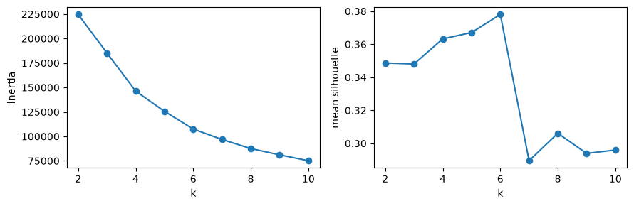
The optimal inertia never increases as k grows (Lesson 4.1), and the inertia printed above falls at every step, so inertia cannot pick k by itself; you look for a bend (the elbow). The silhouette has a maximum. Do the clusters at that k correspond to attacks? The next cell describes each cluster by its size, its share of attacks and the most common service.
km_best = KMeans(n_clusters=best_k, n_init=10, random_state=0).fit(Z_train)
tr = flows[train_mask].reset_index(drop=True).assign(cluster=km_best.labels_)
summary = tr.groupby("cluster").agg(records=("label", "size"), attack_share=("label", "mean"),
                                     top_service=("service", lambda s: s.value_counts().index[0]))
print(summary.round(3))
print()
print(pd.crosstab(tr["cluster"], tr["attack_type"]).to_string())
max_cluster_attack_share = float(summary["attack_share"].max())
min_cluster_attack_share = float(summary["attack_share"].min())
high = summary.index[summary["attack_share"] > 0.10]
in_high = tr["cluster"].isin(high).to_numpy()
high_attack_frac = float(tr.loc[in_high, "label"].sum() / tr["label"].sum())
high_record_frac = float(in_high.mean())
print(f"clusters with more than 10% attacks: {len(high)}; they hold {high_attack_frac:.1%} of the training attacks "
      f"and {high_record_frac:.1%} of the training records")
records attack_share top_service cluster 0 14526 0.004 https 1 5542 0.003 dns 2 610 0.477 other 3 399 0.188 https 4 228 0.531 ssh 5 4970 0.008 smtp attack_type bruteforce dos exfil normal scan cluster 0 1 0 0 14462 63 1 15 0 0 5527 0 2 0 110 0 319 181 3 0 0 75 324 0 4 121 0 0 107 0 5 40 0 2 4928 0 clusters with more than 10% attacks: 3; they hold 80.1% of the training attacks and 4.7% of the training records
The large clusters follow services (web, DNS, mail and remote administration) and contain few attacks. Most attacks fall into a few small clusters, each dominated by one or two attack families, and none of these clusters is pure. k-means groups records that are close in feature space, so each attack family shares its cluster with the benign records that look most like it; section 8 shows which benign behaviors these are.
3. Principal components
PCA on the standardized training features gives the share of variance explained by each component. We report the smallest number of components whose cumulative share reaches 90%.
pca = PCA().fit(Z_train)
evr = pca.explained_variance_ratio_
cum = np.cumsum(evr)
n90 = int(np.searchsorted(cum, 0.90) + 1)
for i, (e, c) in enumerate(zip(evr, cum), 1):
    print(f"PC{i:<2d} {e:.3f}  cumulative {c:.3f}")
print(f"smallest number of components reaching 90%: {n90} (cumulative {cum[n90 - 1]:.3f})")
PC1 0.340 cumulative 0.340 PC2 0.188 cumulative 0.528 PC3 0.135 cumulative 0.663 PC4 0.091 cumulative 0.754 PC5 0.081 cumulative 0.835 PC6 0.044 cumulative 0.879 PC7 0.043 cumulative 0.922 PC8 0.038 cumulative 0.960 PC9 0.030 cumulative 0.990 PC10 0.009 cumulative 0.999 PC11 0.001 cumulative 1.000 smallest number of components reaching 90%: 7 (cumulative 0.922)
Two components are far from 90%, so the 2-D projection below is a picture of part of the data, not a faithful summary. We draw a random sample of 3,000 training records, colored by label.
proj_idx = rng.choice(len(Z_train), 3000, replace=False)
P2 = pca.transform(Z_train[proj_idx])[:, :2]
lab2 = y_train[proj_idx]
fig, ax = plt.subplots(figsize=(6, 4.5))
ax.scatter(P2[lab2 == 0, 0], P2[lab2 == 0, 1], s=4, alpha=0.4, label="normal")
ax.scatter(P2[lab2 == 1, 0], P2[lab2 == 1, 1], s=10, alpha=0.9, label="attack")
ax.set_xlabel("PC1"); ax.set_ylabel("PC2"); ax.legend()
plt.show()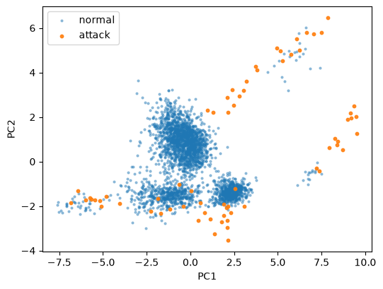
4. DBSCAN on the projection
DBSCAN needs a radius eps and a minimum number of points min_samples. We set min_samples=10 and, following the sorted k-distance heuristic of Ester et al. (1996), compute each point's distance to its 10th nearest neighbor (counting the point itself, as scikit-learn does) and take a high quantile of those distances as eps.
min_samples = 10
nn = NearestNeighbors(n_neighbors=min_samples).fit(P2)
kdist = np.sort(nn.kneighbors(P2)[0][:, -1])
eps = float(np.quantile(kdist, 0.95))
db = DBSCAN(eps=eps, min_samples=min_samples).fit(P2)
db_labels = db.labels_
n_db_clusters = int(len(set(db_labels)) - (1 if -1 in db_labels else 0))
noise = db_labels == -1
print(f"eps = {eps:.3f}, clusters: {n_db_clusters}, noise points: {noise.sum()} of {len(P2)}")
print(f"share of noise among normal records: {noise[lab2 == 0].mean():.3f}")
print(f"share of noise among attack records: {noise[lab2 == 1].mean():.3f}")
print(f"noise points that are normal: {(noise & (lab2 == 0)).sum()}, attacks: {(noise & (lab2 == 1)).sum()}")
dbscan_noise_normal = float(noise[lab2 == 0].mean())
dbscan_noise_attack = float(noise[lab2 == 1].mean())
eps = 0.448, clusters: 3, noise points: 92 of 3000 share of noise among normal records: 0.017 share of noise among attack records: 0.612 noise points that are normal: 51, attacks: 41
Attacks are more likely than normal records to be labeled noise, but most noise points are still normal, because normal records are far more numerous. This pattern returns in every detector below.
5. Three anomaly detectors in two training settings
In the novelty setting each detector is trained on the normal records of days 0 to 9 only. This assumes someone has labeled the training period, which in practice means it has been reviewed. In the contaminated setting it is trained on all records of days 0 to 9, attacks included, as happens when nobody has reviewed the data. Both are scored on days 10 to 13. For every detector a higher score means more anomalous; we use the negative of scikit-learn's score_samples.
The training time of the one-class SVM grows at least quadratically with the number of training records, so it is trained on a random sample of 5,000 records in each setting.
settings = {"novelty": train_mask & (y == 0), "contaminated": train_mask}

def fit_detectors(fit_mask, seed=0):
    X_fit = Z[fit_mask]
    local = np.random.default_rng(seed)
    sub = local.choice(len(X_fit), min(5000, len(X_fit)), replace=False)
    iso = IsolationForest(n_estimators=200, random_state=seed).fit(X_fit)
    lof = LocalOutlierFactor(n_neighbors=20, novelty=True).fit(X_fit)
    ocsvm = OneClassSVM(kernel="rbf", gamma="scale", nu=0.05).fit(X_fit[sub])
    return {"isolation forest": iso, "LOF": lof, "one-class SVM": ocsvm}

scores, models = {}, {}
for setting, mask in settings.items():
    models[setting] = fit_detectors(mask)
    for name, m in models[setting].items():
        scores[(setting, name)] = -m.score_samples(Z_test)

ap = {key: average_precision_score(y_test, s) for key, s in scores.items()}
table = pd.Series(ap).unstack(0)[["novelty", "contaminated"]]
print(table.round(3))
print(f"test base rate (about the AP of a random ranking): {y_test.mean():.3f}")
novelty contaminated LOF 0.471 0.149 isolation forest 0.384 0.406 one-class SVM 0.479 0.350 test base rate (about the AP of a random ranking): 0.041
Compare each row. Contamination of the training data lowers the AP of LOF sharply and that of the one-class SVM less, while the isolation forest scores slightly higher in the contaminated setting. LOF compares the density around a point with the density around its training neighbors. When the training data contains attacks of the same kind, a test attack finds those attacks among its neighbors and no longer looks locally sparse; section 9 shows this most clearly for denial of service.
6. The contamination parameter moves the threshold only
IsolationForest and LocalOutlierFactor take a contamination argument. It does not change the scores; it only sets offset_, the threshold used by predict. With a number, the offset is placed so that this fraction of the training records falls below it; with the default "auto", the isolation forest uses a fixed offset of -0.5. The next cell fits the same forest twice with different values.
fit_x = Z[settings["novelty"]]
iso_auto = IsolationForest(n_estimators=200, random_state=0, contamination="auto").fit(fit_x)
iso_10 = IsolationForest(n_estimators=200, random_state=0, contamination=0.10).fit(fit_x)
same_scores = bool(np.array_equal(iso_auto.score_samples(Z_test), iso_10.score_samples(Z_test)))
alerts_auto = int((iso_auto.predict(Z_test) == -1).sum())
alerts_10 = int((iso_10.predict(Z_test) == -1).sum())
print("identical score_samples:", same_scores)
print(f"offset_: auto {iso_auto.offset_:.4f}, contamination=0.10 {iso_10.offset_:.4f}")
print(f"alerts on the test days: auto {alerts_auto:,}, contamination=0.10 {alerts_10:,}")
identical score_samples: True offset_: auto -0.5000, contamination=0.10 -0.4890 alerts on the test days: auto 995, contamination=0.10 1,205
The ranking, and therefore AP and precision at k, is the same for any value of contamination. Only the number of alerts changes, and it is better chosen from the alert budget than from a guess at the attack rate.
7. Precision at k
An analyst works down the ranked list. Precision at k is the share of attacks among the k highest-scored test records. We compute it for every k from 10 to the number of test attacks; beyond that point it cannot reach 1, because there are not enough attacks to fill the list.
n_attacks_test = int(y_test.sum())
k_grid = np.arange(10, n_attacks_test + 1)

def precision_at_k(score, labels, k_values):
    hits = np.cumsum(labels[np.argsort(-score, kind="stable")])
    return hits[k_values - 1] / k_values

prec_k = {key: precision_at_k(s, y_test, k_grid) for key, s in scores.items()}
fig, ax = plt.subplots(figsize=(7, 3.5))
for (setting, name), p in prec_k.items():
    if setting == "novelty":
        ax.plot(k_grid, p, label=name)
ax.axhline(y_test.mean(), color="gray", ls=":", label="random ranking")
ax.set_xlabel("k (alerts reviewed)"); ax.set_ylabel("precision at k"); ax.legend()
plt.show()
for key, p in prec_k.items():
    print(f"{key[0]:<13} {key[1]:<17} P@50 {p[50 - 10]:.2f}  P@100 {p[100 - 10]:.2f}  P@{n_attacks_test} {p[-1]:.2f}")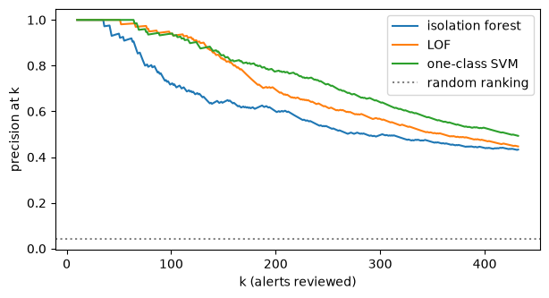
novelty       isolation forest  P@50 0.94  P@100 0.72  P@432 0.43
novelty       LOF               P@50 1.00  P@100 0.94  P@432 0.45
novelty       one-class SVM     P@50 1.00  P@100 0.94  P@432 0.49
contaminated  isolation forest  P@50 0.98  P@100 0.88  P@432 0.44
contaminated  LOF               P@50 0.46  P@100 0.33  P@432 0.21
contaminated  one-class SVM     P@50 0.76  P@100 0.68  P@432 0.41
8. Which benign behaviors receive the highest scores?
The generator in data/make_dataset.py gives each benign behavior a recognizable signature. Backups run at night from the first six hosts of each site and upload large volumes; the misconfigured service runs on hosts 7 to 9 of each site and never receives bytes back; the IT scanner is host A010 on days 3 and 9; administrators use ssh or rdp. The function below recovers the behavior of each normal record from these columns (labels are used only to restrict it to normal records).
def benign_behavior(df):
    host = df["src_host"].str[1:].astype(int).to_numpy()
    svc = df["service"].to_numpy()
    night = df["hour"].isin([0, 1, 2, 3, 4, 23]).to_numpy()
    out = np.full(len(df), "other", dtype=object)
    out[np.isin(svc, ["http", "https"])] = "web"
    out[svc == "dns"] = "dns"
    out[svc == "smtp"] = "mail"
    out[np.isin(svc, ["ssh", "rdp"])] = "admin"
    out[(host <= 6) & night & (df["src_bytes"].to_numpy() > 1e5)] = "backup"
    out[(host >= 7) & (host <= 9) & (df["dst_bytes"].to_numpy() == 0)] = "misconfigured service"
    scanner = ((df["src_host"] == "A010").to_numpy() & df["day"].isin([3, 9]).to_numpy()
               & df["hour"].isin([10, 11, 14]).to_numpy() & (df["dst_host_count"].to_numpy() >= 100)
               & (df["serror_rate"].to_numpy() + df["rerror_rate"].to_numpy() > 0.3))
    out[scanner] = "IT scanner"
    return out

normal_all = flows[flows["label"] == 0]
print(pd.Series(benign_behavior(normal_all)).value_counts())
print()
print("IT scanner records by day:", normal_all[benign_behavior(normal_all) == "IT scanner"]["day"].value_counts().sort_index().to_dict())
print()
print("k-means clusters of section 2 against behavior (training period; attacks by family):")
tr_behavior = np.where(tr["label"] == 1, tr["attack_type"], benign_behavior(tr))
print(pd.crosstab(tr["cluster"], tr_behavior).to_string())
web 20735
dns 7540
mail 4524
admin 2093
backup 452
misconfigured service 226
IT scanner 160
Name: count, dtype: int64
IT scanner records by day: {3: 86, 9: 74}
k-means clusters of section 2 against behavior (training period; attacks by family):
col_0 IT scanner admin backup bruteforce dns dos exfil mail misconfigured service scan web
cluster
0 0 0 0 1 0 0 0 0 0 63 14462
1 0 0 0 15 5378 0 0 72 1 0 76
2 160 0 0 0 0 110 0 0 159 181 0
3 0 0 324 0 0 0 75 0 0 0 0
4 0 107 0 121 0 0 0 0 0 0 0
5 0 1369 0 40 12 0 2 3194 0 0 353
The scanner ran only on days 3 and 9, so it is part of the training period and never appears among the test records. In the novelty setting it is part of what the detectors learn as normal.
The cross-tabulation shows what the attack-heavy k-means clusters of section 2 contain. Each attack family sits next to the benign behavior it resembles, for example exfiltration next to the nightly backups.
An analyst who reviews the ranked test records from the top meets the false alarms in order. We look at as many of the first records of each ranking as there are attacks in the test period and count the behaviors behind the false alarms among them. The last column compares each behavior's share of these false alarms with its share of all normal test records; a ratio above 1 means the detector ranks that behavior higher than its frequency alone would explain.
test_behavior = np.where(y_test == 1, "attack", benign_behavior(test))
normal_share = pd.Series(test_behavior[y_test == 0]).value_counts(normalize=True)
print("share of each behavior among normal test records:")
print(normal_share.round(4).to_dict())
print()
TOP = n_attacks_test
fa_counts = {}
for key, s in scores.items():
    top = np.argsort(-s, kind="stable")[:TOP]
    fa = pd.Series(test_behavior[top][y_test[top] == 0]).value_counts()
    fa_counts[key] = fa.to_dict()
    ratio = (fa / fa.sum() / normal_share.reindex(fa.index)).round(1)
    print(f"{key[0]} / {key[1]}: {int(fa.sum())} false alarms in the top {TOP}")
    print(pd.DataFrame({"count": fa, "ratio to normal share": ratio}).to_string())
    print()
share of each behavior among normal test records:
{'web': 0.5807, 'dns': 0.2137, 'mail': 0.125, 'admin': 0.0613, 'backup': 0.0127, 'misconfigured service': 0.0066}
novelty / isolation forest: 245 false alarms in the top 432
count ratio to normal share
backup 124 39.8
misconfigured service 66 41.1
admin 49 3.3
web 6 0.0
novelty / LOF: 239 false alarms in the top 432
count ratio to normal share
web 138 1.0
mail 35 1.2
dns 30 0.6
admin 25 1.7
backup 8 2.6
misconfigured service 3 1.9
novelty / one-class SVM: 219 false alarms in the top 432
count ratio to normal share
admin 87 6.5
web 50 0.4
misconfigured service 44 30.6
backup 23 8.3
dns 11 0.2
mail 4 0.1
contaminated / isolation forest: 243 false alarms in the top 432
count ratio to normal share
backup 125 40.4
misconfigured service 66 41.4
admin 45 3.0
web 7 0.0
contaminated / LOF: 342 false alarms in the top 432
count ratio to normal share
web 200 1.0
mail 46 1.1
dns 41 0.6
admin 40 1.9
backup 12 2.8
misconfigured service 3 1.3
contaminated / one-class SVM: 253 false alarms in the top 432
count ratio to normal share
admin 79 5.1
web 62 0.4
misconfigured service 38 22.9
mail 26 0.8
backup 25 7.8
dns 23 0.4
The false alarms are not a random sample of normal traffic, and each detector has its own preferences. The isolation forest places almost every backup and misconfigured-service record of the test period among its first records, dozens of times more often than their share of normal traffic would suggest (the ratio column). Administrator connections are the largest group among the one-class SVM's false alarms, and it too ranks the misconfigured service far above its share. LOF behaves differently. Its false alarms follow the ordinary mix of web, mail and DNS traffic, probably because the backups form a dense group of their own and are therefore not locally sparse. Each of these behaviors is unusual in some sense, and an anomaly detector measures only how unusual a record is.
The IT scanner does not appear because it never ran in the test period. It did run in the training period, so in both settings the detectors learned its port-scan-like records as normal.
9. Recall per attack family at an alert budget
Now fix an alert budget of 25 alerts per day, 100 over the four test days. Which attacks do the 100 highest-scored records contain?
BUDGET = 100
families = sorted(test.loc[test["label"] == 1, "attack_type"].unique())
recall_family = {}
for key, s in scores.items():
    top = np.zeros(len(s), bool)
    top[np.argsort(-s, kind="stable")[:BUDGET]] = True
    recall_family[key] = {f: float(top[(test["attack_type"] == f).to_numpy()].mean()) for f in families}
rf = pd.DataFrame(recall_family).T
print(rf.round(2))
bruteforce c2beacon dos exfil scan
novelty isolation forest 0.00 0.00 0.42 0.00 0.59
LOF 0.48 0.06 0.74 0.03 0.07
one-class SVM 0.48 0.00 0.72 0.00 0.21
contaminated isolation forest 0.00 0.00 0.84 0.00 0.53
LOF 0.08 0.13 0.04 0.03 0.00
one-class SVM 0.52 0.00 0.22 0.00 0.16
Recall differs sharply by family and by detector. Every detector trained on clean data finds part of the denial-of-service records, which flood a target with half-open connections. The c2beacon family is new in the test period, the situation anomaly detection is often said to be made for, yet its small, regular connections resemble ordinary web traffic, and the cell above shows how few of them reach the top 100 of any ranking. Being new in the test period did not make these records unusual in feature space.
Try this
- Add
houras a feature and predict what happens to the backup false alarms. Then run it. - Remove the IT scanner records from the novelty training set and refit. Does recall on the
scanfamily rise for any detector? - Change
n_neighborsof LOF from 20 to 100 in the contaminated setting. Does the larger neighborhood dilute the training attacks enough to recover AP? - Set the budget to 25 alerts in total and recompute the per-family recall.
- Fit k-means with k equal to the number of attack families plus one and cross-tabulate the clusters against
attack_type.
Results summary
These are the numbers quoted in the lesson text, and the data used by the figures.
def key_name(setting, name):
    short = {"isolation forest": "iforest", "LOF": "lof", "one-class SVM": "ocsvm"}[name]
    return f"{short}_{setting}"

results = {
    "n_records_raw": int(len(raw)),
    "n_records": int(len(flows)),
    "n_duplicates": int(len(raw) - len(flows)),
    "n_train": int(train_mask.sum()),
    "n_train_attacks": int(y_train.sum()),
    "n_test": int(test_mask.sum()),
    "n_test_attacks": n_attacks_test,
    "n_test_c2beacon": int((test["attack_type"] == "c2beacon").sum()),
    "n_test_dos": int((test["attack_type"] == "dos").sum()),
    "n_test_scan": int((test["attack_type"] == "scan").sum()),
    "n_test_bruteforce": int((test["attack_type"] == "bruteforce").sum()),
    "n_test_exfil": int((test["attack_type"] == "exfil").sum()),
    "test_base_rate": float(y_test.mean()),
    "best_k": int(best_k),
    "best_silhouette": float(max(silhouette)),
    "silhouette_k2": float(silhouette[0]),
    "max_cluster_attack_share": max_cluster_attack_share,
    "min_cluster_attack_share": min_cluster_attack_share,
    "kmeans_high_clusters": int(len(high)),
    "kmeans_high_attack_frac": high_attack_frac,
    "kmeans_high_record_frac": high_record_frac,
    "pca_n90": n90,
    "pca_cum_at_n90": float(cum[n90 - 1]),
    "pca_cum_at_n90_minus1": float(cum[n90 - 2]),
    "pca_evr1": float(evr[0]),
    "pca_evr2": float(evr[1]),
    "pca_cum2": float(cum[1]),
    "dbscan_eps": eps,
    "dbscan_min_samples": min_samples,
    "dbscan_clusters": n_db_clusters,
    "dbscan_noise_normal": dbscan_noise_normal,
    "dbscan_noise_attack": dbscan_noise_attack,
    "dbscan_noise_points": int(noise.sum()),
    "dbscan_noise_normal_n": int((noise & (lab2 == 0)).sum()),
    "dbscan_noise_attack_n": int((noise & (lab2 == 1)).sum()),
    "proj_n_attacks": int(lab2.sum()),
    "if_same_scores": str(same_scores),
    "if_offset_auto": float(iso_auto.offset_),
    "if_offset_10": float(iso_10.offset_),
    "if_alerts_auto": alerts_auto,
    "if_alerts_10": alerts_10,
    "budget": BUDGET,
    "top_reviewed": TOP,
    "normal_share_backup": float(normal_share.get("backup", 0)),
    "n_test_backup": int((test_behavior == "backup").sum()),
    "n_test_misconfig": int((test_behavior == "misconfigured service").sum()),
    "n_test_normal": int((y_test == 0).sum()),
    "normal_share_misconfig": float(normal_share.get("misconfigured service", 0)),
    "normal_share_admin": float(normal_share.get("admin", 0)),
}
for (setting, name), v in ap.items():
    results["ap_" + key_name(setting, name)] = float(v)
for (setting, name), p in prec_k.items():
    kn = key_name(setting, name)
    results[f"p50_{kn}"] = float(p[50 - 10])
    results[f"p100_{kn}"] = float(p[100 - 10])
    results[f"pall_{kn}"] = float(p[-1])
    fa = fa_counts[(setting, name)]
    results[f"fa_{kn}"] = int(sum(fa.values()))
    results[f"fa_backup_{kn}"] = int(fa.get("backup", 0))
    results[f"fa_misconfig_{kn}"] = int(fa.get("misconfigured service", 0))
    results[f"fa_admin_{kn}"] = int(fa.get("admin", 0))
    for f in families:
        results[f"recall_{f}_{kn}"] = recall_family[(setting, name)][f]
for k, v in results.items():
    print(f"{k:<34} {v}")

export = {
    "ks": ks, "inertia": inertia, "silhouette": silhouette,
    "evr": [float(v) for v in evr], "n90": n90,
    "proj": np.round(P2, 4).tolist(), "proj_label": [int(v) for v in lab2],
    "dbscan_label": [int(v) for v in db_labels],
    "k_grid": [int(v) for v in k_grid],
    "prec_k": {key_name(*key): [round(float(v), 5) for v in p] for key, p in prec_k.items()},
    "ap": {key_name(*key): float(v) for key, v in ap.items()},
    "false_alarms": {key_name(*key): {k: int(v) for k, v in d.items()} for key, d in fa_counts.items()},
    "recall_family": {key_name(*key): d for key, d in recall_family.items()},
    "families": families,
    "normal_share": {k: float(v) for k, v in normal_share.items()},
}

# When the course build runs this notebook, it saves the numbers for the lesson pages.
if os.environ.get("COURSE_RESULTS"):
    import json
    with open(os.environ["COURSE_RESULTS"], "w") as f:
        json.dump({"results": results, "data": export}, f)
n_records_raw 37873 n_records 36770 n_duplicates 1103 n_train 26275 n_train_attacks 608 n_test 10495 n_test_attacks 432 n_test_c2beacon 180 n_test_dos 50 n_test_scan 86 n_test_bruteforce 83 n_test_exfil 33 test_base_rate 0.041162458313482614 best_k 6 best_silhouette 0.37805634904788266 silhouette_k2 0.3486594787358801 max_cluster_attack_share 0.5307017543859649 min_cluster_attack_share 0.0027066041140382533 kmeans_high_clusters 3 kmeans_high_attack_frac 0.8009868421052632 kmeans_high_record_frac 0.04707897240723121 pca_n90 7 pca_cum_at_n90 0.9219042050222169 pca_cum_at_n90_minus1 0.8790457135825618 pca_evr1 0.34037847593682063 pca_evr2 0.18751117505108986 pca_cum2 0.5278896509879105 dbscan_eps 0.4483907048277632 dbscan_min_samples 10 dbscan_clusters 3 dbscan_noise_normal 0.017388339584043642 dbscan_noise_attack 0.6119402985074627 dbscan_noise_points 92 dbscan_noise_normal_n 51 dbscan_noise_attack_n 41 proj_n_attacks 67 if_same_scores True if_offset_auto -0.5 if_offset_10 -0.48904789825991857 if_alerts_auto 995 if_alerts_10 1205 budget 100 top_reviewed 432 normal_share_backup 0.012719864851435954 n_test_backup 128 n_test_misconfig 66 n_test_normal 10063 normal_share_misconfig 0.006558680314021664 normal_share_admin 0.06131372354168737 ap_iforest_novelty 0.3837173539107467 ap_lof_novelty 0.4710041558065307 ap_ocsvm_novelty 0.47942762051892707 ap_iforest_contaminated 0.4062713085949329 ap_lof_contaminated 0.14917305823929491 ap_ocsvm_contaminated 0.3497234974965128 p50_iforest_novelty 0.94 p100_iforest_novelty 0.72 pall_iforest_novelty 0.43287037037037035 fa_iforest_novelty 245 fa_backup_iforest_novelty 124 fa_misconfig_iforest_novelty 66 fa_admin_iforest_novelty 49 recall_bruteforce_iforest_novelty 0.0 recall_c2beacon_iforest_novelty 0.0 recall_dos_iforest_novelty 0.42 recall_exfil_iforest_novelty 0.0 recall_scan_iforest_novelty 0.5930232558139535 p50_lof_novelty 1.0 p100_lof_novelty 0.94 pall_lof_novelty 0.44675925925925924 fa_lof_novelty 239 fa_backup_lof_novelty 8 fa_misconfig_lof_novelty 3 fa_admin_lof_novelty 25 recall_bruteforce_lof_novelty 0.4819277108433735 recall_c2beacon_lof_novelty 0.05555555555555555 recall_dos_lof_novelty 0.74 recall_exfil_lof_novelty 0.030303030303030304 recall_scan_lof_novelty 0.06976744186046512 p50_ocsvm_novelty 1.0 p100_ocsvm_novelty 0.94 pall_ocsvm_novelty 0.4930555555555556 fa_ocsvm_novelty 219 fa_backup_ocsvm_novelty 23 fa_misconfig_ocsvm_novelty 44 fa_admin_ocsvm_novelty 87 recall_bruteforce_ocsvm_novelty 0.4819277108433735 recall_c2beacon_ocsvm_novelty 0.0 recall_dos_ocsvm_novelty 0.72 recall_exfil_ocsvm_novelty 0.0 recall_scan_ocsvm_novelty 0.20930232558139536 p50_iforest_contaminated 0.98 p100_iforest_contaminated 0.88 pall_iforest_contaminated 0.4375 fa_iforest_contaminated 243 fa_backup_iforest_contaminated 125 fa_misconfig_iforest_contaminated 66 fa_admin_iforest_contaminated 45 recall_bruteforce_iforest_contaminated 0.0 recall_c2beacon_iforest_contaminated 0.0 recall_dos_iforest_contaminated 0.84 recall_exfil_iforest_contaminated 0.0 recall_scan_iforest_contaminated 0.5348837209302325 p50_lof_contaminated 0.46 p100_lof_contaminated 0.33 pall_lof_contaminated 0.20833333333333334 fa_lof_contaminated 342 fa_backup_lof_contaminated 12 fa_misconfig_lof_contaminated 3 fa_admin_lof_contaminated 40 recall_bruteforce_lof_contaminated 0.08433734939759036 recall_c2beacon_lof_contaminated 0.12777777777777777 recall_dos_lof_contaminated 0.04 recall_exfil_lof_contaminated 0.030303030303030304 recall_scan_lof_contaminated 0.0 p50_ocsvm_contaminated 0.76 p100_ocsvm_contaminated 0.68 pall_ocsvm_contaminated 0.41435185185185186 fa_ocsvm_contaminated 253 fa_backup_ocsvm_contaminated 25 fa_misconfig_ocsvm_contaminated 38 fa_admin_ocsvm_contaminated 79 recall_bruteforce_ocsvm_contaminated 0.5180722891566265 recall_c2beacon_ocsvm_contaminated 0.0 recall_dos_ocsvm_contaminated 0.22 recall_exfil_ocsvm_contaminated 0.0 recall_scan_ocsvm_contaminated 0.16279069767441862