Unit 4 · Lesson 4.3
Anomaly detection and the alert budget
Supervised detectors learn what attacks look like from labeled examples, so they recognize attacks that resemble ones already labeled. Anomaly detection instead learns what normal traffic looks like and scores each new record by how far it departs from that model, in the hope that attacks, including unseen ones, depart further than benign activity. This lesson presents three widely used detectors (isolation forest, local outlier factor and the one-class support vector machine), shows how their scores become alerts and how to evaluate them against an alert budget, and examines the assumption on which all of them rest. That assumption, that malicious means unusual, fails in both directions in security data, and the lab measures how often.
Two settings: clean and contaminated training data
What the training data contains matters as much as the algorithm. Scikit-learn distinguishes two settings. In novelty detection the training data is assumed to contain no anomalies, and the detector is asked whether new records resemble it. In outlier detection the training data itself contains anomalies, and the detector must model the dense regions while ignoring the stragglers. Chandola et al. (2009) call the first setting semisupervised, because it needs labels for the normal class, and the second unsupervised; unsupervised techniques assume that normal instances are far more frequent than anomalies and suffer from a high false alarm rate when that is not true.
In security, clean training data means a reviewed period, which is expensive and may still contain missed attacks. Sommer and Paxson (2010) list the difficulty of obtaining attack-free training data among the well-recognized problems of anomaly detection, together with numerous false positives and attackers who teach a system to accept malicious activity by introducing it gradually. Training on contaminated data is therefore common, and Lab 4 measures its cost by training every detector both ways on days 0 to 9 and testing on days 10 to 13.
Isolation forest
Liu et al. (2008) built a detector on the observation that anomalies are few and different, so they are easier to separate from the rest of the data than normal points are. An isolation tree is grown on a random subsample of the training data by repeatedly choosing a feature at random and a split value uniformly between that feature's minimum and maximum in the current node, until each point is alone or a height limit is reached. The path length \(h(x)\) of a point is the number of edges from the root to the leaf where it ends. A point in a sparse region is isolated after a few splits; a point deep inside a dense cluster needs many. Figure 4.7 shows one tree's splits for each case.
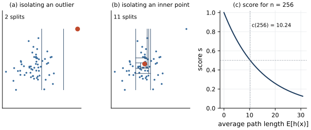
Figure 4.7. Isolation by random axis-parallel splits, on 61 synthetic points drawn by the figure script. (a) The splits of one random isolation tree until the red outlier is alone. (b) The splits of a tree until a point near the center of the cloud is alone; many more are needed. (c) The anomaly score of equation \eqref{eq:iforest} as a function of the average path length for subsamples of n = 256; the score is 0.5 when the average path length equals c(256), marked by the dotted lines.
Path lengths grow with the size of the subsample, so they are normalized by the average path length of an unsuccessful search in a binary search tree built on \(n\) points,
where \(H(i)\) is the \(i\)-th harmonic number and 0.5772156649 is Euler's constant. The anomaly score of \(x\) is
where \(\mathbb{E}[h(x)]\) is the average path length of \(x\) over the trees of the forest (Liu et al., 2008). If the average path length equals \(c(n)\), the score is 0.5. Scores near 1 indicate anomalies, and scores well below 0.5 indicate normal points. Liu et al. found that subsamples of 256 points and 100 trees generally sufficed, and that subsampling reduces two effects, swamping, the labeling of normal points as anomalies when they lie close to anomalies, and masking, the hiding of anomalies by other anomalies clustered near them.
For a worked example with \(n = 256\), \(H(255) \approx \ln 255 + 0.5772\), which is 6.1185, so \(c(256) \approx 12.237 - 1.992\), which is 10.245. A point isolated after 4 splits on average scores \(2^{-4/10.245} \approx 0.763\), and one needing 15 splits scores \(2^{-15/10.245} \approx 0.362\).
In scikit-learn, IsolationForest.score_samples returns the opposite of \(s\), so lower means more anomalous. The labs use its negative, so that higher always means more anomalous.
Local outlier factor
A record can be unusual relative to its neighborhood without being far from everything. Breunig et al. (2000) give the example of a point just outside a dense cluster, closer to that cluster than many points of a sparse cluster are to each other. A global distance threshold cannot flag it without also flagging the sparse cluster. The local outlier factor (LOF) compares the density around a point with the density around its neighbors.
Let \(m\) be the number of neighbors (n_neighbors in scikit-learn, MinPts in the paper), \(N_m(p)\) the \(m\) nearest neighbors of \(p\), and \(d_m(o)\) the distance from \(o\) to its \(m\)-th nearest neighbor. The reachability distance of \(p\) from \(o\), written \(r_m(p, o)\), is \(\max\{d_m(o), d(p, o)\}\), which smooths distances to points inside dense neighborhoods. The local reachability density of \(p\) is the inverse of its average reachability distance from its neighbors,
and the local outlier factor averages the ratio of the neighbors' densities to that of \(p\),
For a point inside a cluster of roughly uniform density, LOF is close to 1; Breunig et al. prove bounds that make this precise. A point whose neighbors are much denser than itself has LOF well above 1. They suggested at least 10 neighbors, because the statistic fluctuates for smaller values. Duplicated records are a practical hazard. If a point has at least \(m\) exact copies, its reachability distances can all be zero and its density infinite, which is one more reason to remove the collector duplicates of the course data before fitting.
By default scikit-learn's LocalOutlierFactor only scores the data it was fitted on. To score new records, as in both settings of the lab, it must be created with novelty=True.
The one-class support vector machine
Schölkopf et al. (2001) adapted the support vector machine to data from one class. Records are mapped into a feature space by a kernel, usually the radial basis function (RBF) kernel \(K(x, x') = \exp(-\gamma \lVert x - x' \rVert^2)\), and the method finds a hyperplane that separates the mapped training data from the origin with maximum margin, allowing some training points to fall on the wrong side. The decision function has the form \(f(x) = \sum_i \alpha_i K(x_i, x) - \rho\), positive on the estimated support of the data and negative outside, and the training points with \(\alpha_i > 0\) are the support vectors. A parameter \(\nu \in (0, 1]\) controls the trade-off. Their \(\nu\)-property states that, when the solution has \(\rho \ne 0\), \(\nu\) is an upper bound on the fraction of training points that fall outside (the outliers) and a lower bound on the fraction of training points that are support vectors, and that both fractions approach \(\nu\) asymptotically, with probability 1, for data from a distribution without discrete components and an analytic kernel such as the RBF kernel.
Because \(\nu\) bounds the fraction of training points treated as outliers, it should reflect how contaminated the training data may be, not the attack rate expected in deployment. The kernel parameter \(\gamma\), which sets how quickly similarity decays with distance (Lesson 3.2), matters as much. A large \(\gamma\) wraps the boundary tightly around each training point, and a small one draws a smooth blob. Training slows as the training set grows, because the method works with kernel values between pairs of training points, which is why Lab 4 trains the one-class SVM on a random sample of 5,000 records in each setting.
Show the answer
With \(c(256) \approx 10.245\), record A scores \(2^{-5/10.245} \approx 0.713\) and record B scores \(2^{-20/10.245} \approx 0.258\). Record A is isolated in fewer splits and has the higher score, so it is the more anomalous of the two. Record B needed far more splits than an average record and looks normal.
From scores to alerts with the contamination parameter
Each detector produces a score, and an alert requires a threshold. IsolationForest and LocalOutlierFactor accept a contamination argument, which is easily mistaken for an assumption that must match the true attack rate. The scores returned by score_samples do not depend on it. It only sets the attribute offset_, the threshold used by predict and subtracted by decision_function. With the default "auto", the offset is fixed (−0.5 for the isolation forest, which flags records with \(s > 0.5\), and −1.5 for LOF). With a number such as 0.05, the offset is placed at the corresponding percentile of the training scores, so that 5% of the training records are flagged.
Lab 4 fits the same forest twice, with the default and with contamination=0.10. The test scores are identical (np.array_equal returns True), and only the threshold changes, from -0.500 to -0.489, which raises the number of alerts on the four test days from 995 to 1,205. Because the ranking does not change, neither does any ranking metric such as AP. The one-class SVM differs here, because \(\nu\) enters the optimization and changes the fitted function itself.
A threshold derived from the training data says how many training records would have been flagged. A security team needs a threshold that matches the number of alerts it can investigate per day, the alert budget defined in Lesson 1.2 and used to choose a threshold in Lesson 2.3. The direct way to honor the budget is to rank the records of a period by score and alert on the top \(k\), where \(k\) is the budget for that period, or to set the threshold at the \(k\)-th highest score of a recent period of the same length.
Evaluating against a budget: AP and precision at k
Average precision (AP, Lesson 2.3) summarizes the whole ranking. When the budget is fixed, the more direct measure is precision at k, the share of attacks among the \(k\) highest-scored records,
where \(A\) is the number of attacks in the evaluated period. The bound holds because there are only \(A\) attacks to place in the list; for \(k > A\), even a perfect ranking has precision \(A/k\). A random ranking has expected precision equal to the base rate at every \(k\). Precision at k can also be measured in deployment, where labels are missing, because estimating it requires investigating only the top \(k\) records, which the alerts trigger anyway. Recall requires knowing how many attacks were missed, which a periodic review of a random sample of unflagged records can estimate.
The test period of Lab 4 contains 10,495 records, of which 432 are attacks (a base rate of 4.1%). Figure 4.8 shows the AP of the three detectors in both settings.
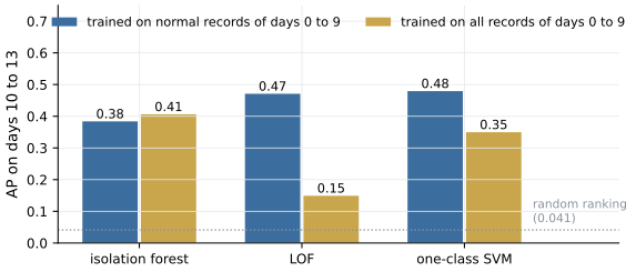
Figure 4.8. Average precision on the test days (10 to 13) of Lab 4 for three detectors, each trained on the normal records of days 0 to 9 (novelty setting, blue) or on all records of days 0 to 9 (contaminated setting, gold). The dotted line is the test base rate, approximately the AP of a random ranking. Eleven standardized flow features; the one-class SVM is trained on 5,000 sampled records.
Trained on clean data, the one-class SVM (AP 0.479) and LOF (0.471) rank attacks better than the isolation forest (0.384). Trained on contaminated data, LOF falls to 0.149 and becomes the worst of the three, the one-class SVM falls to 0.350, and the isolation forest rises slightly to 0.406, moving from last place to first. LOF judges a record by its neighbors. When the training data contains earlier attacks of the same kind, a test attack finds them among its neighbors and no longer looks locally sparse. The isolation forest, which grows each tree on a small random subsample, was not harmed by the contamination in this data. Figure 4.9 shows precision at k for every k from 10 to 432.
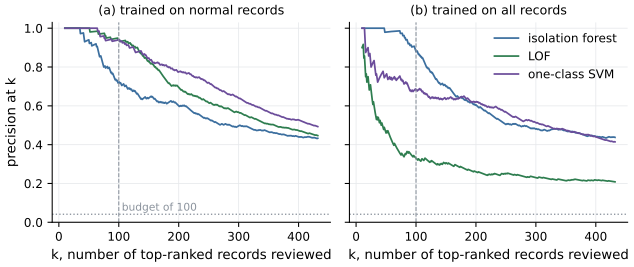
Figure 4.9. Precision at k, equation \eqref{eq:patk}, on the test days of Lab 4 for k from 10 to the number of test attacks, for the three detectors trained (a) on normal records only and (b) on all records of days 0 to 9. The dashed vertical line marks a budget of 100 alerts over the four test days; the dotted horizontal line is the base rate, the expected precision of a random ranking.
With a budget of 100 alerts over the four days, 25 a day, the detectors trained on clean data reach precision 0.94 (LOF), 0.94 (one-class SVM) and 0.72 (isolation forest), far above the base rate. The choice of detector and training data matters most at the top of the list, which is the only part an analyst sees.
Show the answer
A perfect ranking puts all 400 attacks first, so the top 1,000 contain 400 attacks and \(P@1000 = 400/1000 = 0.4\), the bound \(A/k\) of equation \eqref{eq:patk}. A random ranking has expected precision equal to the base rate, \(400/20{,}000 = 0.02\), at every \(k\).
Unusual is not malicious
Every detector in this lesson measures how unlike the training data a record is. Sommer and Paxson (2010) note that anomaly detection systems report what has not been seen before, whether benign or not, instead of identifying malicious behavior, and argue that a detector that cannot bridge the gap between abnormal activity and attacks is unlikely to meet operational expectations. The gap runs both ways.
Rare benign activity produces alerts. The course data contains such activity on purpose (nightly backups that upload large volumes, a misconfigured service that retries a closed port, administrators who mistype passwords, an IT vulnerability scanner). Lab 4 recovers the behavior behind each normal record and counts the false alarms among the first 432 records of each ranking, as many as there are test attacks; Figure 4.10 shows the detectors trained on clean data. The isolation forest places 124 of the 128 backup records and 66 of the 66 misconfigured-service records of the test period in that list, although these two behaviors make up only 1.3% and 0.7% of normal test traffic. Administrator connections are the largest group among the one-class SVM's false alarms (87 of 219, against 6.1% of normal test traffic), and it also lists 44 misconfigured-service records. LOF's false alarms follow the ordinary mix of web, DNS and mail traffic, probably because the backups form a dense group of their own and are therefore not locally unusual. Each detector has its own notion of unusual, and each includes benign behavior. The IT scanner does not appear because it ran only on days 3 and 9, inside the training period.
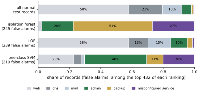
Figure 4.10. Composition of the false alarms among the top 432 test records of each detector trained on normal records of days 0 to 9 (Lab 4), compared with the composition of all normal test records (top bar). Behaviors are recovered from the generating features of data/make_dataset.py. Percentages of 7% or more are printed. The isolation forest's false alarms consist almost entirely of backups, the misconfigured service and administrator connections, while those of LOF resemble normal traffic as a whole.
Attacks that resemble normal traffic are missed. Chandola et al. (2009) note that when anomalies result from malicious actions, adversaries often adapt to make the anomalous observations appear normal, and that normal behavior keeps evolving. The test period of Lab 4 contains a command-and-control family, c2beacon, that never occurs in the training period, the situation in which anomaly detection is often said to excel. The table below gives the recall of each attack family within the budget of 100 alerts, for the detectors trained on clean data.
| Family | Test records | Isolation forest | LOF | One-class SVM |
|---|---|---|---|---|
| dos | 50 | 0.42 | 0.74 | 0.72 |
| scan | 86 | 0.59 | 0.07 | 0.21 |
| bruteforce | 83 | 0.00 | 0.48 | 0.48 |
| exfil | 33 | 0.00 | 0.03 | 0.00 |
| c2beacon | 180 | 0.00 | 0.06 | 0.00 |
All three detectors find part of the denial-of-service records, which flood a target with half-open connections. Exfiltration, whose large uploads resemble the nightly backups, is almost never in the top 100, and the new c2beacon family, whose small, regular check-ins look like ordinary web traffic, is caught only by LOF and only rarely, so being new did not make it unusual. The detectors also disagree with each other. The isolation forest finds scans but no brute-force attempts, while LOF and the one-class SVM find brute-force attempts and fewer scans.
No single detector wins
That disagreement is not peculiar to this dataset. Han et al. (2022) benchmarked 30 anomaly detection algorithms on 57 tabular datasets in ADBench and found that none of the unsupervised methods was statistically better than the others. Performance depended on whether a method's assumptions matched the type of anomaly; LOF, for example, was best on local anomalies in their simulations but performed poorly on clustered anomalies. Their results concern tabular benchmark datasets and synthetic anomaly types, mostly scored with the area under the ROC curve, but the conclusion serves as a working rule for network traffic too. Choose a detector by evaluating it on data and attacks like the ones you expect, on a time-ordered split, and report precision at the budget and per-family recall in addition to AP, because an average can hide a family that is never found. When a detector's top alerts are dominated by a benign behavior, look first to domain knowledge, for example an allow-list for the backup schedule, a separate model per host role, or a feature that distinguishes the benign behavior from the attack it resembles.
Show the answer
The contamination parameter of IsolationForest does not change score_samples; it only sets the threshold offset_. AP depends only on the ranking of the scores, so it is identical for every value of contamination when the forest is fitted with the same data and random_state. An AP difference must come from something else, such as a different random seed or different training data. The 3% figure also confuses two quantities. The parameter describes the share of training records to be flagged, while the attack rate in deployment is unknown and changes over time. A threshold is better set from the alert budget.
What the lab shows
Lab 4
Clustering and anomaly detection on network flows
Open in ColabRead with outputsNotebook on GitHubAbout 1 minute to run on a laptop CPU
Sections 1 and 5 to 9 of Lab 4 produce every result of this lesson; the "Try this" suggestions at the end vary the features, the training data and the budget.
Summary
Anomaly detectors score records by how unlike the training data they are. The isolation forest normalizes the average number of random splits needed to isolate a record by \(c(n)\), giving a score of 0.5 for an average record. LOF compares a record's local density with that of its neighbors, and the one-class SVM estimates the support of the training data, with \(\nu\) bounding the fraction of training outliers from above and of support vectors from below. In the lab, contamination of the training data cost LOF most of its ranking quality. Scikit-learn's contamination parameter moves only the threshold, which is better set from the alert budget, and detectors are best compared by precision at that budget and by per-family recall. Because unusual is not the same as malicious, rare benign behavior fills the top of the list while attacks that resemble normal traffic, including a family never seen before, are missed, so anomaly scores need domain knowledge and a realistic evaluation before they drive alerts.
References
- Breunig, M. M., Kriegel, H.-P., Ng, R. T., and Sander, J. (2000). LOF: Identifying density-based local outliers. Proceedings of the 2000 ACM SIGMOD International Conference on Management of Data, 93-104. https://doi.org/10.1145/342009.335388
- Chandola, V., Banerjee, A., and Kumar, V. (2009). Anomaly detection: A survey. ACM Computing Surveys, 41(3), 15:1-15:58. https://doi.org/10.1145/1541880.1541882
- Han, S., Hu, X., Huang, H., Jiang, M., and Zhao, Y. (2022). ADBench: Anomaly detection benchmark. Advances in Neural Information Processing Systems 35 (NeurIPS 2022), Datasets and Benchmarks Track, 32142-32159. https://doi.org/10.52202/068431-2329
- Liu, F. T., Ting, K. M., and Zhou, Z.-H. (2008). Isolation forest. 2008 Eighth IEEE International Conference on Data Mining, 413-422. https://doi.org/10.1109/ICDM.2008.17
- Schölkopf, B., Platt, J. C., Shawe-Taylor, J., Smola, A. J., and Williamson, R. C. (2001). Estimating the support of a high-dimensional distribution. Neural Computation, 13(7), 1443-1471. https://doi.org/10.1162/089976601750264965
- Sommer, R., and Paxson, V. (2010). Outside the closed world: On using machine learning for network intrusion detection. 2010 IEEE Symposium on Security and Privacy, 305-316. https://doi.org/10.1109/SP.2010.25