Unit 4 · Lesson 4.1
Clustering
A security team rarely has labels for most of what it collects. Alerts arrive faster than analysts can triage them, malware repositories receive more samples than anyone can reverse-engineer, and the inventory of what each host actually does is usually out of date. Clustering groups records that resemble each other without being told what the groups should be. It can reduce ten thousand alerts to a few dozen groups for an analyst to review, or show that a new sample behaves like a known family, but it cannot say which group is malicious. This lesson develops k-means in detail, then density-based methods (DBSCAN and HDBSCAN) and hierarchical clustering, and closes with what clusters do and do not tell you about attacks.
The k-means objective
Let \(x_1, \dots, x_n \in \mathbb{R}^d\) be the records, each a vector of \(d\) numeric features, and let \(k\) be the number of clusters, chosen in advance. A clustering assigns each record \(x_i\) to a cluster \(c(i) \in \{1, \dots, k\}\), and cluster \(j\) is summarized by a center \(\mu_j \in \mathbb{R}^d\). The k-means objective, also called the within-cluster sum of squares or inertia, is
the total squared Euclidean distance from each record to the center of its cluster. Small \(J\) means compact clusters. Finding the allocation and centers that minimize \(J\) exactly is NP-hard, even with two clusters, as Arthur and Vassilvitskii (2007) note, so every practical method is a heuristic.
For fixed centers, \(J\) is minimized by assigning each record to its nearest center. For a fixed allocation, it is minimized by placing each center at the mean of its records, because the mean minimizes the sum of squared distances to a set of points. Alternating these two steps gives Lloyd's algorithm, which is what most software means by k-means:
- choose \(k\) initial centers;
- assign every record to its nearest center;
- move every center to the mean of the records assigned to it;
- repeat steps 2 and 3 until the allocation no longer changes.
Lloyd (1982) derived these two conditions, the center of mass of each region and the boundary halfway between neighboring centers, for the optimal quantization of a one-dimensional signal, and proposed alternating between them; the paper notes that the work was presented in part in 1957. Neither step can increase \(J\), and there are finitely many allocations, so the algorithm stops after finitely many iterations (Arthur and Vassilvitskii, 2007). It stops at a configuration where both conditions hold, which need not be the global minimum. Lloyd already observed that the conditions are necessary but not sufficient, and that several local minima can exist.
A k-means iteration by hand
Take six records in two dimensions, (1, 1), (1, 2), (2, 1), (4, 3), (5, 4) and (4, 4), and \(k = 2\) with the poorly chosen initial centers \(\mu_1 = (1, 1)\) and \(\mu_2 = (2, 1)\). Figure 4.1 shows the three stages.
The first allocation step compares squared distances. The record (1, 2) is at squared distance 1 from \(\mu_1\) and 2 from \(\mu_2\), so it joins cluster 1. The record (4, 3) is at 13 from \(\mu_1\) and 8 from \(\mu_2\), so it joins cluster 2, and so do (5, 4) and (4, 4). Cluster 1 is {(1, 1), (1, 2)} and cluster 2 is {(2, 1), (4, 3), (5, 4), (4, 4)}, with \(J = 0 + 1 + 0 + 8 + 18 + 13 = 40\).
The update step moves the centers to the means, \(\mu_1 = (1, 1.5)\) and \(\mu_2 = (3.75, 3)\), and \(J\) falls to 11.25. In the second allocation step, (2, 1) is at squared distance 1.25 from the new \(\mu_1\) and 7.0625 from \(\mu_2\), so it changes cluster, and \(J\) falls to 5.4375. The second update gives \(\mu_1 = (4/3, 4/3)\) and \(\mu_2 = (13/3, 11/3)\) with \(J = 12/9 + 12/9 \approx 2.667\). A third allocation step changes nothing, and the algorithm stops.
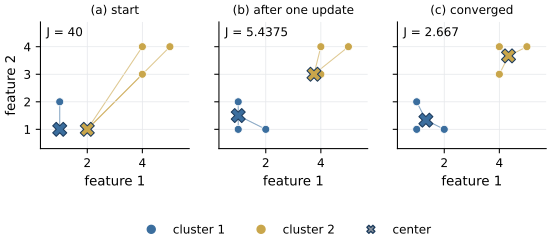
Figure 4.1. Lloyd's algorithm on six points with k = 2, the worked example of this lesson. Points are colored by their current cluster, crosses mark the centers, and thin lines join each point to its center. (a) The initial centers (1, 1) and (2, 1) and the first allocation, J = 40. (b) After the first update the centers are (1, 1.5) and (3.75, 3), and the point (2, 1) has been reassigned, J = 5.4375. (c) After the second update, J = 2.667, and the next allocation changes nothing. J is the objective of equation \eqref{eq:kmeans}.
Here the bad start cost only an extra iteration. On larger data it can leave the algorithm in a poor local minimum, for example with two centers sharing one natural group while another center covers two groups.
Better starting points with k-means++
Arthur and Vassilvitskii (2007) proposed a randomized seeding. The first center is a record chosen uniformly at random. Each further center is a record \(x\) chosen with probability proportional to \(D(x)^2\), the squared distance from \(x\) to the nearest center chosen so far, so far-away records are likely to become centers and records close to an existing center almost never do. They proved that the expected objective after seeding alone satisfies
where \(J_{\mathrm{opt}}\) is the optimal value, and Lloyd's iterations can only lower \(J\) further. In the worked example, suppose the first center is (1, 1). The squared distances of the other five records to it are 1, 1, 13, 25 and 18, which sum to 58, so the second center is (5, 4) with probability \(25/58 \approx 0.43\) and one of the three upper-right records with probability \(56/58 \approx 0.97\). The poor start of the worked example, two centers among the three lower-left records, has probability \(2/58\).
Scikit-learn's KMeans uses this seeding by default and, with n_init, runs the whole algorithm several times from different seeds and keeps the run with the lowest \(J\). Fix random_state when you need reproducible clusters.
Show the answer
The optimal inertia never increases when \(k\) grows, because a solution with \(k\) clusters can be turned into one with \(k + 1\) by splitting any cluster, which cannot increase the sum of squared distances. With \(k = n\) every record is its own center and \(J = 0\). Minimizing \(J\) over \(k\) would always choose the largest \(k\). One looks instead for a bend where further clusters bring little reduction (the elbow), or uses a criterion such as the silhouette, which penalizes clusters that are close to each other.
What k-means assumes
Because \(J\) sums squared Euclidean distances to a single center, k-means prefers clusters that are roughly spherical and of similar spread and size. A long thin cluster is cut into pieces, and a cluster that wraps around another cannot be found at all. The method has no notion of noise. Every record is assigned to some cluster, so a single extreme record either pulls a center toward it or claims a center of its own.
The distances also depend on how features are scaled. A byte count in the millions next to a rate between 0 and 1 makes the rate irrelevant to every distance. This unit uses the remedy of Lesson 2.1, a log transform for heavy-tailed counts followed by standardization, with the scaling statistics computed on the training data only.
Choosing k with the silhouette
Rousseeuw (1987) proposed the silhouette to judge how well each record sits in its cluster. For record \(i\) in cluster \(A\), let \(a(i)\) be its average distance to the other members of \(A\), and let \(b(i)\) be the smallest, over all other clusters \(C\), of its average distance to the members of \(C\). The silhouette of \(i\) is
which lies between \(-1\) and 1. Values near 1 mean the record is much closer to its own cluster than to the nearest other one, values near 0 mean it lies between two clusters, and negative values suggest it was assigned to the wrong cluster. A record that is alone in its cluster gets \(s(i) = 0\) by convention. Rousseeuw suggested choosing the \(k\) for which the average silhouette over all records is largest.
In the worked example after convergence, the record (2, 1) has average distance \(a = (1 + \sqrt{2})/2 \approx 1.207\) to the other two members of its cluster and average distance \(b \approx 3.559\) to the other cluster, the mean of \(\sqrt{8}\), \(\sqrt{18}\) and \(\sqrt{13}\), so \(s = (3.559 - 1.207)/3.559\), about 0.661. Averaged over all six records the silhouette is about 0.70. Computing the silhouette requires all pairwise distances, so on large data it is estimated on a random sample.
Figure 4.2 shows both criteria for k-means on the 26,275 training records of Lab 4, described by eleven standardized features. The inertia falls at every step without a sharp elbow (a value of \(k\) after which further clusters bring little reduction), which is common on real data. The silhouette is highest at \(k = 6\), with a value of 0.38, which indicates clusters that overlap considerably.
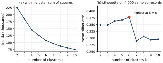
Figure 4.2. k-means on the 26,275 deduplicated training records of Lab 4 (days 0 to 9, eleven standardized features, seven of them log-transformed), for k from 2 to 10. (a) The inertia, equation \eqref{eq:kmeans}, in thousands; it decreases with k and shows no sharp elbow. (b) The mean silhouette, equation \eqref{eq:silhouette}, computed on a random sample of 4,000 records; the red point marks its maximum.
At this \(k\), the share of attacks per cluster ranges from 0.3% to 53.1%. The large clusters follow services (web, DNS, and mail with remote administration) and contain few attacks. The 3 clusters in which attacks exceed 10% of the members hold 80% of the training attacks but only 4.7% of the records, and none of them is pure. Denial of service and scans share a cluster with the misconfigured service and the IT scanner, exfiltration shares one with the nightly backups, and brute-force attempts share one with administrator logins. The clusters describe kinds of behavior, whether benign or malicious. A cluster with a high attack share is a lead for an analyst to follow; turning it into a detector would require labels and an evaluation on held-out data (Lesson 2.2).
Density-based clustering with DBSCAN
Ester et al. (1996) defined clusters as regions of high density separated by regions of low density, with an algorithm called DBSCAN. It has two parameters, a radius \(\varepsilon\) (eps in scikit-learn) and a count \(m\) (min_samples). The \(\varepsilon\)-neighborhood of a record \(p\) is the set of records within distance \(\varepsilon\) of \(p\), including \(p\) itself. Three kinds of record follow:
- a core point has at least \(m\) records in its \(\varepsilon\)-neighborhood;
- a border point is not a core point but lies in the \(\varepsilon\)-neighborhood of one;
- a noise point is neither, and belongs to no cluster.
Two core points within \(\varepsilon\) of each other belong to the same cluster, and chains of such links connect a whole cluster; border points join the cluster of a nearby core point. DBSCAN does not need \(k\), finds clusters of arbitrary shape, and labels outlying records as noise (label \(-1\) in scikit-learn) instead of forcing them into a cluster. Panels (a) and (b) of Figure 4.3 show the difference on two interleaved half-moons, which k-means cuts with a straight boundary and DBSCAN separates.
To choose the parameters, Ester et al. proposed the sorted k-dist graph, which here plots the distance from every record to its \(m\)-th nearest neighbor, sorted in decreasing order. With this \(m\), a threshold on this graph is a candidate for \(\varepsilon\), since records whose distance is equal to or smaller than the threshold then become core points; for two-dimensional data they fixed \(m = 4\). The same \(\varepsilon\) and \(m\) apply to every cluster, chosen to match the least dense one, and Ester et al. noted that two nearby clusters of different density may be merged. Panel (c) shows the other side of the problem. With an \(\varepsilon\) that suits a dense cluster, a sparse cluster nearby falls apart into fragments and noise.
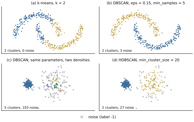
Figure 4.3. Synthetic two-dimensional data, made by the figure script with fixed seeds. Top, 400 points on two interleaved half-moons. (a) k-means with k = 2 splits them with a straight boundary. (b) DBSCAN with eps = 0.15 and min_samples = 5 recovers both moons. Bottom, a dense cluster of 250 points next to a sparse cluster of 150 points. (c) DBSCAN with the same parameters keeps the dense cluster but breaks the sparse one into several small clusters and many noise points. (d) HDBSCAN with min_cluster_size = 20 finds both clusters. Gray crosses are noise points (label -1); colors distinguish clusters within each panel only.
HDBSCAN
HDBSCAN removes the single global density threshold; Campello et al. (2015) describe it in detail. For a count \(m_{\mathrm{pts}}\), which plays the role of DBSCAN's \(m\), the core distance of a record is the distance to its \(m_{\mathrm{pts}}\)-th nearest neighbor, counting the record itself, which is the smallest \(\varepsilon\) at which the record would be a core point. The mutual reachability distance between records \(p\) and \(q\) is the largest of the two core distances and the distance between \(p\) and \(q\). Applying a variant of DBSCAN's rule, in which clusters are formed by core points alone, at every possible \(\varepsilon\) gives a hierarchy of clusters, which HDBSCAN computes from a minimum spanning tree of the mutual reachability graph. It then selects a flat set of clusters from the hierarchy by maximizing a measure of cluster stability, so that different clusters may correspond to different density levels. Panel (d) of Figure 4.3 shows the result on the two-density data.
Scikit-learn has included HDBSCAN since version 1.3. Its main parameter is min_cluster_size, the smallest group you are willing to call a cluster, which in a security setting states how many related events you need before they are worth an analyst's attention.
Show the answer
Its \(\varepsilon\)-neighborhood contains four records including itself, fewer than five, so it is not a core point. It lies within \(\varepsilon\) of a core point, so it is a border point and joins that core point's cluster. Halving eps shrinks every neighborhood. The record may then lose its link to the core point, and the core point may itself stop being a core point, so the record can become noise. Smaller eps produces more noise and smaller or more fragmented clusters.
Hierarchical clustering
Agglomerative hierarchical clustering starts with every record as its own cluster and repeatedly merges the two closest clusters until one remains. The result is a tree, the dendrogram, which can be cut at any height to obtain a flat clustering. The distance between clusters is set by the linkage. Single linkage uses the closest pair of members and can follow long chains, complete linkage uses the farthest pair, average linkage the mean over all pairs, and Ward's method merges the pair whose merger increases the within-cluster sum of squares \eqref{eq:kmeans} the least. Standard implementations need all pairwise distances and do not scale to millions of records. Bayer et al. (2009) addressed this for malware. They converted execution traces into behavioral profiles and used locality-sensitive hashing to compute an approximate single-linkage clustering of more than 75,000 samples in less than three hours.
Clustering in security work
Grouping alerts lets an analyst investigate one representative of a group and close the rest when it proves benign, or escalate the group together. Grouping malware by behavior, as Bayer et al. did, separates samples of known families from new behavior. Grouping hosts by their connection patterns reveals roles. Tan et al. (2003) grouped the hosts of two enterprise networks by whom they communicate with and found up to two orders of magnitude fewer groups than hosts, groups that reflected the logical structure of each network.
The same caveats apply to every such use. The clusters depend on the features, their scaling and the distance, and the algorithm will produce clusters even from data that has none. A cluster tells you that records are similar, not why. An attacker who imitates benign behavior lands in a benign cluster, and in the course dataset a share of each attack family was generated that way, with its features blended toward the benign traffic it imitates. Clusters also drift as the network changes. In Lab 4, DBSCAN on the first two principal components labels 61% of the sampled attack records as noise but only 1.7% of the normal ones; even so, 51 of the 92 noise points are normal, because normal records are so much more numerous. Small rates applied to a large benign population are the theme of Lesson 1.2, and they return with the anomaly detectors of Lesson 4.3.
Show the answer
The cluster was found without labels, and 25% of its members were benign, so the rule would produce false alerts at that rate or worse. Future runs of k-means can produce different clusters (another seed, another \(k\), drift in the data), so the cluster is not a stable definition. Attacks outside this cluster would be ignored, including any attacker who shapes traffic to look like a benign cluster. If labels are available, a supervised detector trained and evaluated on a time-ordered split (Lesson 2.2) is the right tool; the cluster is useful as a lead and as a candidate feature.
What the lab shows
Lab 4
Clustering and anomaly detection on network flows
Open in ColabRead with outputsNotebook on GitHubAbout 1 minute to run on a laptop CPU
Lab 4 fits the scaling on days 0 to 9 only and never uses label, attack_type or ticket_opened as features. Besides the k-means runs above, it projects the data on two principal components (Lesson 4.2) and runs DBSCAN there with min_samples = 10 and eps = 0.45, the 95th percentile of the distances to the 10th nearest neighbor, counting the record itself (the convention of min_samples), which gives 3 clusters.
Summary
k-means minimizes the within-cluster sum of squares by alternating nearest-center allocation and mean updates. No step increases the objective, so the algorithm converges, but only to a local minimum that depends on the starting centers; k-means++ seeding makes poor starts unlikely and carries an expected \(O(\log k)\) approximation guarantee. The method assumes compact, similarly spread clusters, assigns every record and depends on feature scaling. The optimal inertia can only fall as \(k\) grows, so \(k\) is chosen from an elbow or from the mean silhouette. DBSCAN defines clusters by density, finds arbitrary shapes and labels noise, but its single density threshold fails when clusters differ in density, which HDBSCAN addresses by selecting stable clusters from the whole density hierarchy. In security work clusters organize alerts, samples and hosts for analysts, and they describe similarity of behavior, not maliciousness.
References
- Arthur, D., and Vassilvitskii, S. (2007). k-means++: The advantages of careful seeding. Proceedings of the Eighteenth Annual ACM-SIAM Symposium on Discrete Algorithms (SODA 2007), 1027-1035. https://theory.stanford.edu/~sergei/papers/kMeansPP-soda.pdf
- Bayer, U., Milani Comparetti, P., Hlauschek, C., Kruegel, C., and Kirda, E. (2009). Scalable, behavior-based malware clustering. Network and Distributed System Security Symposium (NDSS 2009). https://www.ndss-symposium.org/wp-content/uploads/2017/09/bay.pdf
- Campello, R. J. G. B., Moulavi, D., Zimek, A., and Sander, J. (2015). Hierarchical density estimates for data clustering, visualization, and outlier detection. ACM Transactions on Knowledge Discovery from Data, 10(1), 5:1-5:51. https://doi.org/10.1145/2733381
- Ester, M., Kriegel, H.-P., Sander, J., and Xu, X. (1996). A density-based algorithm for discovering clusters in large spatial databases with noise. Proceedings of the Second International Conference on Knowledge Discovery and Data Mining (KDD-96), 226-231. AAAI Press. https://cdn.aaai.org/KDD/1996/KDD96-037.pdf
- Lloyd, S. P. (1982). Least squares quantization in PCM. IEEE Transactions on Information Theory, 28(2), 129-137. https://doi.org/10.1109/TIT.1982.1056489
- Rousseeuw, P. J. (1987). Silhouettes: A graphical aid to the interpretation and validation of cluster analysis. Journal of Computational and Applied Mathematics, 20, 53-65. https://doi.org/10.1016/0377-0427(87)90125-7
- Tan, G., Poletto, M., Guttag, J., and Kaashoek, F. (2003). Role classification of hosts within enterprise networks based on connection patterns. Proceedings of the General Track: 2003 USENIX Annual Technical Conference, 15-28. https://www.usenix.org/legacy/event/usenix03/tech/full_papers/tan/tan.pdf