Unit 3 · Lesson 3.2
Nearest neighbors, support vector machines and naive Bayes
The three classifiers of this lesson rest on three different ideas. A nearest-neighbor classifier labels a record like the training records closest to it. A support vector machine places a boundary as far as possible from the nearest records of both classes. Naive Bayes estimates how probable each class makes the observed features and applies Bayes' rule. Each idea has a characteristic strength and a characteristic way to fail on security data, and Lab 3a compares all three on the same intrusion data, while Lab 3b builds phishing URL detectors from naive Bayes and logistic regression.
k-nearest neighbors
The \(k\)-nearest-neighbor (k-NN) classifier stores the training set. To classify a new record \(\mathbf{x}\), it finds the \(k\) training records closest to \(\mathbf{x}\) under a distance such as the Euclidean distance \(\lVert\mathbf{x} - \mathbf{x}'\rVert_2\), and predicts the majority label among them. The share of attacks among the \(k\) neighbors serves as a score,
where \(N_k(\mathbf{x})\) is the set of indices of the \(k\) nearest training records and \(y_i \in \{0, 1\}\) is the label of record \(i\), with 1 for attack. Suppose the five nearest neighbors of a connection lie at distances 0.20, 0.35, 0.40, 0.60 and 0.90 and their labels are attack, normal, attack, normal, normal. With \(k = 3\) the score is \(2/3\) and the connection is flagged at a threshold of 0.5; with \(k = 5\) it is \(2/5\) and it is not. When each of the five neighbors is weighted by the inverse of its distance, the two attacks receive a total weight of \(1/0.2 + 1/0.4 = 7.5\) and all five neighbors a total weight of
so the weighted score is \(7.5/13.13 = 0.571\), because the closest neighbor is an attack.
The Euclidean distance is one member of the Minkowski family. The Minkowski distance between two records with \(d\) features is the norm \(\lVert\mathbf{x} - \mathbf{x}'\rVert_r\) of their difference, where for a vector \(\mathbf{u}\) with components \(u_1, \dots, u_d\) and an exponent \(r \ge 1\),
The case \(r = 2\) is the Euclidean distance, and \(r = 1\) gives the Manhattan distance \(\sum_j |x_j - x'_j|\), the sum of the absolute differences. Scikit-learn's KNeighborsClassifier uses the Minkowski distance with \(r = 2\) by default, set by its parameter p.
The number of neighbors \(k\) controls the tradeoff of Lesson 3.1. With \(k = 1\) the boundary follows every training record, including mislabeled ones, so the variance is high. A large \(k\) averages over a wide region and blurs real structure, so the bias is high. It is chosen on validation data. With two classes an odd \(k\) also rules out ties in the vote, because an odd number of votes cannot split into two equal halves. With \(k = 4\), a vote of two against two needs a rule to break it. Scikit-learn's KNeighborsClassifier then returns the class that comes first in its sorted list of classes, which with labels 0 for normal and 1 for attack is normal. With unlimited data, even \(k = 1\) is surprisingly good. Cover and Hart (1967) proved that, as the training set grows, the error rate of the one-nearest-neighbor rule is bounded above by twice the Bayes error rate, the smallest error achievable by any rule.
A worked example shows how the scales of the features decide which neighbors are nearest. A detector with \(k = 3\) classifies connections to a Secure Shell (SSH) server from two features, the number of failed login attempts in the connection (failed_logins) and the number of bytes the client sent (src_bytes). The table below lists five labeled training connections and a new one. The numbers are invented for teaching. The new connection has five failed logins, between the counts of the two attacks, and no normal connection has more than one, so it evidently belongs with the attacks.
| Record | Class | Failed logins | Bytes sent |
|---|---|---|---|
| A | attack | 6 | 750 |
| B | attack | 4 | 850 |
| C | normal | 0 | 1,150 |
| D | normal | 1 | 1,300 |
| E | normal | 0 | 2,950 |
| new | ? | 5 | 1,200 |
On the raw features, the squared Euclidean distance from the new connection \(\mathbf{x}\) to record C, \(\lVert\mathbf{x} - \mathbf{x}_C\rVert_2^2\), is
and the distance is \(\sqrt{2{,}525} \approx 50.2\). The failed logins contribute 25 of the 2,525 under the square root, so the distance is almost exactly the difference in bytes, and the same holds for the other records. The second table below gives all five distances. Sorted by raw distance, the neighbors are C, D, B, A and E. The three nearest, C, D and B, vote two to one for normal, the score \eqref{eq:knn} is 1/3, and the detector passes a connection with five failed logins as normal.
Now standardize each feature with the mean and the standard deviation of the five training connections (Lesson 2.1). For failed logins they are 2.2 and 2.4, and for bytes sent 1,400 and 800, with the standard deviation computed by dividing by \(n = 5\), as scikit-learn's StandardScaler does. The new connection is scaled with the same training statistics. In the difference of two standardized values the means cancel, so the distance after scaling divides each difference by the standard deviation \(\sigma_j\) of its feature,
where \(z_j = (x_j - \mu_j)/\sigma_j\) is the standardized value of feature \(j\) and \(\mu_j\) its training mean. For record B the squared distance after scaling is
and the distance is \(\sqrt{0.365} \approx 0.604\). A difference of one failed login now weighs as much as a difference of about 333 bytes (800/2.4), where before it weighed as much as one byte. The table below gives the distances from the new connection on the raw and on the standardized features, with the rank of each record in parentheses.
| Record | Class | Raw (rank) | Scaled (rank) |
|---|---|---|---|
| A | attack | 450.0 (4) | 0.700 (2) |
| B | attack | 350.0 (3) | 0.604 (1) |
| C | normal | 50.2 (1) | 2.084 (4) |
| D | normal | 100.1 (2) | 1.671 (3) |
| E | normal | 1,750.0 (5) | 3.021 (5) |
Sorted by scaled distance, the neighbors are B, A, D, C and E. The three nearest, B, A and D, vote two to one for attack, the score is 2/3, and the connection is flagged. Scaling changed the prediction because it changed what the distance measures. Scikit-learn confirms both predictions. The pipeline fits the scaler on the training records only and applies the same transformation to the new one,
import numpy as np
from sklearn.neighbors import KNeighborsClassifier
from sklearn.pipeline import make_pipeline
from sklearn.preprocessing import StandardScaler

X = np.array([[6, 750], [4, 850], [0, 1150], [1, 1300], [0, 2950]])
y = np.array([1, 1, 0, 0, 0])  # 1 attack, 0 normal
new = np.array([[5, 1200]])
raw = KNeighborsClassifier(n_neighbors=3).fit(X, y)
scaled = make_pipeline(StandardScaler(),
                       KNeighborsClassifier(n_neighbors=3)).fit(X, y)
print(raw.predict(new), scaled.predict(new))
dist, idx = scaled[-1].kneighbors(scaled[0].transform(new))
print(idx, dist.round(3))
The first line printed is [0] [1], normal on the raw features and attack after scaling. The second gives the indices of the three scaled neighbors, [[1 0 3]] (records B, A and D), and their distances, 0.604, 0.700 and 1.671.
Show the answer
With \(k = 1\) only the nearest record votes. That is C on the raw features, so the prediction is normal, and B on the scaled features, so the prediction is attack. With \(k = 5\) all five training records vote, three normal against two attacks, so both detectors predict normal. They would predict normal for any new connection, because when \(k\) equals the number of training records every query has the same neighbors. This is the extreme of high bias, and since normal records are the majority in security data, a large \(k\) pulls predictions toward normal.
Three properties matter in practice. First, distances are only meaningful if the features are on comparable scales (Lesson 2.1). In the example the raw distance was almost a difference in bytes, and the same happens in unscaled flow data. Second, k-NN is a lazy learner. Training only stores the data, and every prediction searches it, so prediction cost and memory grow with the training set, which matters for a detector that must score millions of connections a day. Third, in high dimensions distances lose contrast. Figure 3.5 shows that for random points the nearest and the farthest neighbor of a query become almost equally far as the dimension grows, so "nearest" carries less information. This is one face of the curse of dimensionality. Real data often lies near a lower-dimensional structure, which is why k-NN still works on many problems, but the effect is one reason it struggles with thousands of sparse text features.
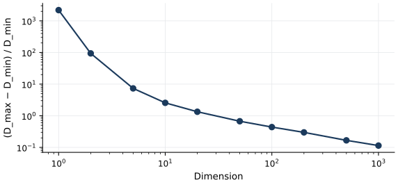
Figure 3.5. Relative contrast of distances, \((D_{\max} - D_{\min})/D_{\min}\), where \(D_{\max}\) and \(D_{\min}\) are the largest and the smallest Euclidean distance from a random query point to 1,000 random points drawn uniformly from the unit cube, as a function of the dimension \(d\) (both axes logarithmic). Each point is the median over 20 queries. In low dimensions the farthest point is many times farther from the query than the nearest; in a thousand dimensions the two are almost equally far. Simulation with a fixed seed.
A stored training set has security consequences of its own. The model is the data, so anyone who can query it learns about the training records (Unit 8 discusses membership inference), and a few poisoned training records near an attack can label it as normal for every future query that lands nearby.
Show the answer
The squared Euclidean distance is a sum of squared differences, and differences in src_bytes are many orders of magnitude larger than differences in the other two features, so the neighbors are simply the records with the most similar byte counts. Standardize the features on the training data, and take \(\log(1 + x)\) of the byte count first, so that a difference of one standard deviation in any feature counts about the same.
Support vector machines
A linear classifier predicts with the sign of \(f(\mathbf{x}) = \mathbf{w}^\top\mathbf{x} + b\). For the SVM, write the labels as \(y_i \in \{-1, +1\}\). If the training data is linearly separable, many hyperplanes separate it; the support vector machine (SVM) chooses the one with the largest margin. The distance from a point \(\mathbf{x}_i\) to the hyperplane is \(|f(\mathbf{x}_i)|/\lVert\mathbf{w}\rVert\). After \(\mathbf{w}\) and \(b\) are rescaled so that the closest points satisfy \(y_i f(\mathbf{x}_i) = 1\), the margin, the width of the empty band between the classes, is
the expression derived by Cortes and Vapnik (1995). Maximizing the margin is the same as minimizing \(\tfrac{1}{2}\lVert\mathbf{w}\rVert^2\) subject to \(y_i(\mathbf{w}^\top\mathbf{x}_i + b) \ge 1\) for every \(i\), a convex quadratic program. For \(\mathbf{w} = (3, 4)\), \(\lVert\mathbf{w}\rVert = 5\) and the margin is 0.4. The training points on the edges of the band are the support vectors; the solution depends on them alone.
Security data is rarely separable, since attacks imitate normal traffic and labels contain errors. Cortes and Vapnik extended the method to non-separable data with slack variables \(\xi_i \ge 0\) that let point \(i\) violate the margin, at a cost controlled by a constant \(C\). In the form used by scikit-learn the problem is
subject to \(y_i(\mathbf{w}^\top\mathbf{x}_i + b) \ge 1 - \xi_i\) and \(\xi_i \ge 0\) for every \(i\). This is equivalent to minimizing \(\tfrac{1}{2}\lVert\mathbf{w}\rVert^2\) plus \(C\sum_i \max(0, 1 - y_i f(\mathbf{x}_i))\). The term \(\max(0, 1 - y f)\) is the hinge loss. A point beyond the margin on the correct side, with \(y f = 1.5\), costs nothing; a point inside the margin but correctly classified, with \(y f = 0.3\), costs 0.7; a misclassified point with \(y f = -0.5\) costs 1.5. A large \(C\) punishes violations and fits the training data closely, while a small \(C\) tolerates them in exchange for a wider margin, so \(C\) plays the same role as in logistic regression. Figure 3.6 draws the margin, the support vectors and three margin violations.
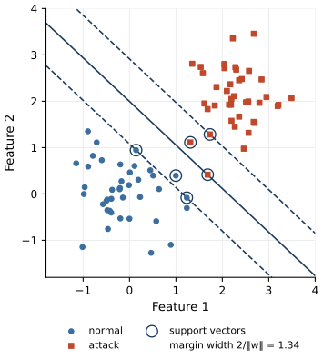
Figure 3.6. A soft-margin linear SVM on two synthetic classes drawn from neighboring normal distributions (blue, normal; red, attack). The solid line is the decision boundary \(f(\mathbf{x}) = 0\), the dashed lines are \(f(\mathbf{x}) = \pm 1\), and the band between them has width \(2/\lVert\mathbf{w}\rVert\). Circled points are support vectors, the records on or inside the margin; the circled points inside the band violate the margin, and only the support vectors determine the boundary. Fitted with scikit-learn's SVC(kernel="linear", C=1).
The kernel trick
The solution of \eqref{eq:softmargin} can be written as \(f(\mathbf{x}) = \sum_i \alpha_i y_i\, \mathbf{x}_i^\top\mathbf{x} + b\), with weights \(\alpha_i\) that are nonzero only for support vectors, and the optimization itself needs the data only through inner products \(\mathbf{x}_i^\top\mathbf{x}_j\). Replace every inner product with a kernel function \(K(\mathbf{u}, \mathbf{v})\) that equals an inner product \(\phi(\mathbf{u})^\top\phi(\mathbf{v})\) in some feature space, and the SVM becomes a linear classifier in that space, which is a nonlinear classifier in the original one. The point is that \(K\) is computed directly from \(\mathbf{u}\) and \(\mathbf{v}\), without ever constructing \(\phi(\mathbf{u})\). Cortes and Vapnik, building on earlier work, describe this as interchanging the order of operations. Instead of mapping vectors into the feature space and taking an inner product there, one compares the vectors in input space and applies a nonlinear function to the result. Mercer's condition characterizes the functions \(K\) for which such a feature space exists.
A small case shows the identity. For two-dimensional inputs, the polynomial kernel \(K(\mathbf{u}, \mathbf{v}) = (\mathbf{u}^\top\mathbf{v} + 1)^2\) equals the inner product under the six-dimensional map
For \(\mathbf{u} = (1, 2)\) and \(\mathbf{v} = (3, 0)\), the kernel gives \((3 + 1)^2 = 16\), and the long way gives
The kernel needed one two-dimensional inner product.
The radial basis function (RBF) kernel,
corresponds to a feature space of infinite dimension, so the explicit map could not be computed at all. The parameter \(\gamma > 0\) sets how quickly similarity decays with distance. With \(\gamma = 0.5\), the two points above, at squared distance 8, have similarity \(e^{-4} = 0.018\). A large \(\gamma\) makes every training point influence only its immediate surroundings and produces a wiggly boundary that can fit noise; a small \(\gamma\) gives a smooth one. Scikit-learn's default, gamma="scale", sets \(\gamma\) to one over the number of features times the variance of the training data. \(C\) and \(\gamma\) interact and are tuned together on validation data. Because the kernel is a function of distances, RBF SVMs need scaled features as much as k-NN does.
A kernel makes a more flexible boundary possible; it does not guarantee that the classes become separable. On overlapping data the soft margin is still needed, and \(C\) still trades training errors for margin. Two practical limits matter for detectors. Training a kernel SVM scales between quadratically and cubically with the number of records, which is why Lab 3a uses an SVM on tens of thousands of records but not on millions. And the output \(f(\mathbf{x})\) is a score proportional to the signed distance from the boundary, not a probability; Platt scaling (Lesson 2.3) was introduced to turn it into one.
Show the answer
Both toward smaller values. A large \(\gamma\) lets each support vector affect only a tiny neighborhood, so the boundary can wrap around individual training records, and a large \(C\) makes the optimizer pay heavily for every training error, so it uses that flexibility. Lowering \(\gamma\) smooths the boundary and lowering \(C\) accepts some training errors for a wider margin, which reduces variance at the cost of some bias.
Naive Bayes
Bayes' rule gives the probability of class \(c\) given features \(\mathbf{x} = (x_1, \dots, x_d)\),
The class-conditional distribution \(P(\mathbf{x} \mid c)\) has too many parameters to estimate directly. Naive Bayes assumes that the features are conditionally independent given the class,
The assumption is about independence within each class, not overall. In URL data the tokens paypal and login are strongly correlated across all URLs, because both are frequent in phishing URLs; the assumption only requires that, among phishing URLs, knowing one does not change the probability of the other, and likewise among legitimate URLs. That is still usually false, but less false than unconditional independence.
Different models for \(P(x_j \mid c)\) give different variants. Gaussian naive Bayes models each numeric feature with a normal distribution per class. Multinomial naive Bayes, the standard choice for text, treats a document as a sequence of word draws from a class-specific distribution over the vocabulary. McCallum and Nigam (1998) compared it with the multivariate Bernoulli model, which records only the presence or absence of each word, and found that the multinomial model usually performs better at large vocabulary sizes. They estimate the probability of word \(t\) in class \(c\) with a Laplace prior that adds one to every count,
where \(N_{tc}\) is the number of occurrences of \(t\) in the training documents of class \(c\) and \(|V|\) is the size of the vocabulary. Without the added one, a word never seen in one class would give that class a probability of exactly zero for every document containing it, whatever the other words say.
Here is a worked example. A filter is trained on 100 phishing and 900 legitimate URLs, so the prior odds of phishing are \(100/900 = 0.111\). The phishing URLs contain 600 tokens and the legitimate ones 5,400, over a vocabulary of 2,000 tokens. A new URL contains the tokens paypa1, verify and login, with the training counts in the table below.
| Token | Phishing | Legitimate |
|---|---|---|
paypa1 |
4 | 0 |
verify |
45 | 3 |
login |
60 | 90 |
By \eqref{eq:laplace}, the smoothed probability of a token is one plus its count in the class, divided by 2,600 in the phishing class and by 7,400 in the legitimate class, where each denominator adds the vocabulary size of 2,000 to the token total of the class. For paypa1 these are \(5/2{,}600 = 0.00192\) and \(1/7{,}400 = 0.000135\). The next table gives both smoothed probabilities of each token, \(\hat P(t \mid \text{phish})\) under Phishing and \(\hat P(t \mid \text{legit})\) under Legitimate, and their ratio.
| Token | Phishing | Legitimate | Ratio |
|---|---|---|---|
paypa1 |
0.00192 | 0.000135 | 14.2 |
verify |
0.0177 | 0.000541 | 32.7 |
login |
0.0235 | 0.0123 | 1.91 |
Under \eqref{eq:naive}, the posterior odds are the prior odds times the product of the ratios, which with the unrounded ratios is
so the posterior probability of phishing is \(98.7/99.7 = 0.990\). In practice the products are computed as sums of logarithms to avoid numerical underflow. The token login contributes little, because legitimate sites have login pages too.
Naive Bayes trains in one pass over the data and handles very large vocabularies, which made it the classical spam filter. Sahami et al. (1998) cast junk-mail filtering as a decision problem with asymmetric costs and classified a message as junk only when its probability exceeded 99.9%, because discarding a legitimate message is far worse than letting junk through. They also noted that they did not expect naive Bayes, because of its independence assumption, to give very accurate probability estimates. That observation is general. Domingos and Pazzani (1997) showed that the classifier can be optimal under zero-one loss (the misclassification rate) even when the independence assumption is violated by a wide margin, while its probability estimates are optimal under quadratic loss only if the assumption holds. Correlated evidence is counted more than once, which pushes the posterior toward 0 or 1, the distortion that Niculescu-Mizil and Caruana (2005) observed for naive Bayes. The ranking, and so the AP, can be good while the probabilities are overconfident, and they need recalibration before they are used with a cost-based threshold (Lesson 2.3).
Show the answer
Without smoothing, the estimate \(\hat P(\texttt{paypa1} \mid \text{legit})\) is \(0/5{,}400 = 0\), so the likelihood of the URL under the legitimate class is zero. Because its other tokens all occur in phishing training URLs, the posterior probability of phishing is exactly 1, whatever their counts. Conversely, a token never seen in phishing training URLs sets the phishing likelihood to zero, so the posterior is exactly 0 for any URL whose tokens all occur in legitimate training URLs. A URL with tokens of both kinds has two zero likelihoods and no defined posterior. An attacker who adds a single token that occurred only in legitimate training data, such as the name of a common news site, could then make any phishing URL without a phishing-only token score zero. Smoothing keeps every token's evidence finite.
The three models on the course data
Lab 3a trains k-NN with \(k = 25\), an RBF SVM with the default \(C = 1\) and \(\gamma\), and Gaussian naive Bayes on the time-ordered split of flows.csv, with log-transformed and standardized features. Their AP on the test days is 0.571, 0.613 and 0.310 respectively, against 0.518 for logistic regression. Gaussian naive Bayes is weakest here, probably because several features are far from normal within each class (failed_logins is a small count, and the error rates pile up at 0) and because the features are strongly dependent within each class.
Figure 3.7 shows how the models carve up two of the features, the logarithm of count and serror_rate. Scans and denial-of-service attacks produce many connections with many SYN errors, the IT scanner produces many connections with a moderate error rate, and ordinary traffic produces few connections and few errors.
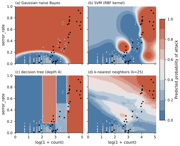
Figure 3.7. Predicted probability of attack (shading, from blue for 0 to red for 1) of four models trained on two features of the training days of Lab 3a, \(\log(1 + \text{count})\) on the horizontal axis and serror_rate on the vertical axis. The models are fitted on a random sample of 6,000 training records, and the dots show 1,500 of them (black, attack; white, normal). k-NN and the decision tree follow the data locally, the tree with axis-parallel steps; the RBF SVM draws a smooth curved boundary; Gaussian naive Bayes fits one normal distribution per class and feature, which gives a quadratic boundary. Data from Lab 3a.
Lab 3b turns to text. On the synthetic URLs of urls.csv, multinomial naive Bayes on word counts reaches an AP of 0.996 and logistic regression on character n-gram TF-IDF weights 0.998, averaged over five random splits; neither raises a false alert at a threshold of 0.5, and their recall at that threshold is 0.959 and 0.964. These numbers are high because the URLs are built from a few templates; on real URL feeds, Ma et al. (2009) reported accuracies of 95 to 99% with lexical and host-based features. The more useful output of the lab is the list of n-grams with the largest weights in Figure 3.8.
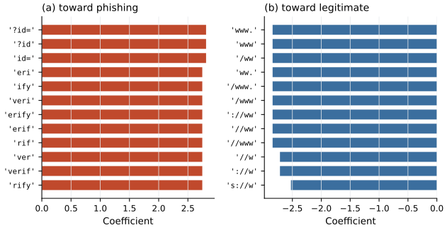
Figure 3.8. The character n-grams with the largest positive weights (toward phishing, red) and the largest negative weights (toward legitimate, blue) in the logistic regression of Lab 3b, trained on character 3- to 5-gram TF-IDF features of the synthetic URLs. N-grams that always occur together, such as the overlapping pieces of verify, receive identical weights, so a run of bars of equal length is one pattern. Several patterns, such as ?id= and www., are artifacts of the templates that generated the data. Data from Lab 3b.
The top phishing n-grams include the query string ?id=, which the templates add only to phishing URLs, and the top legitimate n-grams include www., which the templates add only to legitimate ones. The model has learned how the data was made, which Arp et al. (2022) call a spurious correlation, and an attacker can remove the query string at no cost, which takes that evidence out of the score. Inspecting weights is a cheap way to find such shortcuts, and it is one advantage of linear models and naive Bayes over less transparent ones.
What the labs show
Lab 3a
Comparing classifiers on a time-ordered split
Open in ColabRead with outputsNotebook on GitHubAbout 3 minutes to run on a laptop CPU
Lab 3b
Detecting phishing URLs from their text
Open in ColabRead with outputsNotebook on GitHubAbout 1 minute to run on a laptop CPU
Summary
k-NN labels a record by its nearest training records. Without scaling, the feature with the largest numeric range decides the distance, so k-NN needs scaled features. It also needs a choice of \(k\) that balances bias and variance, odd when there are two classes so that votes cannot tie, and a search over the stored data at prediction time, and its distances lose contrast in high dimensions. A support vector machine maximizes the margin \(2/\lVert\mathbf{w}\rVert\), uses slack variables and the hinge loss for overlapping classes, and through kernels computes inner products in a high- or infinite-dimensional feature space without mapping the data there; \(C\) and \(\gamma\) control its flexibility, and its scores are not probabilities. Naive Bayes applies Bayes' rule under the assumption that features are independent within each class, needs smoothing to avoid zero probabilities, and can classify well even when the assumption fails, but its probabilities are overconfident. On security text, inspecting what the model weighs most is a quick test for shortcuts that an attacker could exploit.
References
- Arp, D., Quiring, E., Pendlebury, F., Warnecke, A., Pierazzi, F., Wressnegger, C., Cavallaro, L., and Rieck, K. (2022). Dos and don'ts of machine learning in computer security. Proceedings of the 31st USENIX Security Symposium, 3971-3988. https://www.usenix.org/conference/usenixsecurity22/presentation/arp
- Cortes, C., and Vapnik, V. (1995). Support-vector networks. Machine Learning, 20(3), 273-297. https://doi.org/10.1007/BF00994018
- Cover, T. M., and Hart, P. E. (1967). Nearest neighbor pattern classification. IEEE Transactions on Information Theory, 13(1), 21-27. https://doi.org/10.1109/TIT.1967.1053964
- Domingos, P., and Pazzani, M. (1997). On the optimality of the simple Bayesian classifier under zero-one loss. Machine Learning, 29(2-3), 103-130. https://doi.org/10.1023/A:1007413511361
- Ma, J., Saul, L. K., Savage, S., and Voelker, G. M. (2009). Beyond blacklists: Learning to detect malicious web sites from suspicious URLs. Proceedings of the 15th ACM SIGKDD International Conference on Knowledge Discovery and Data Mining, 1245-1254. https://doi.org/10.1145/1557019.1557153
- McCallum, A., and Nigam, K. (1998). A comparison of event models for naive Bayes text classification. Learning for Text Categorization: Papers from the 1998 Workshop, AAAI Technical Report WS-98-05, 41-48. https://cdn.aaai.org/Workshops/1998/WS-98-05/WS98-05-007.pdf
- Niculescu-Mizil, A., and Caruana, R. (2005). Predicting good probabilities with supervised learning. Proceedings of the 22nd International Conference on Machine Learning, 625-632. https://doi.org/10.1145/1102351.1102430
- Sahami, M., Dumais, S., Heckerman, D., and Horvitz, E. (1998). A Bayesian approach to filtering junk e-mail. Learning for Text Categorization: Papers from the 1998 Workshop, AAAI Technical Report WS-98-05, 55-62. https://cdn.aaai.org/Workshops/1998/WS-98-05/WS98-05-009.pdf