Unit 3 · Lesson 3.1
Linear and logistic regression
Linear models are the first models to try on a new security problem, and they are easy to explain to an auditor. They train in seconds, their parameters can be read, and they set the baseline that any more complex detector must beat. Comparing a new detector only with other complex models, without such a simple baseline, is one of the ten pitfalls identified by Arp et al. (2022). This lesson develops linear regression and logistic regression from their loss functions, shows how they are fitted in closed form or by gradient descent, works a simple regression and one gradient step by hand, introduces L2 and L1 regularization and the tradeoff between bias and variance, and explains what the coefficients of a logistic regression do and do not tell you about a detector.
Linear regression and the normal equation
A linear regression predicts a real number from a feature vector \(\mathbf{x} \in \mathbb{R}^d\) as \(\hat y = \mathbf{w}^\top\mathbf{x} + b\), with a weight vector \(\mathbf{w} \in \mathbb{R}^d\) and an intercept \(b\). Security examples are predicting the duration of a transfer from its size, or the expected number of connections a host makes in the next hour. Given \(n\) training pairs \((\mathbf{x}_i, y_i)\), the parameters are chosen to minimize the mean squared error (MSE),
Absorb the intercept into the weights by adding a constant feature 1 to every \(\mathbf{x}_i\), and stack the vectors as the rows of an \(n \times (d+1)\) matrix \(X\), with the targets in a vector \(\mathbf{y}\). The loss becomes \(\frac{1}{n}\lVert \mathbf{y} - X\boldsymbol{\theta}\rVert^2\) with \(\boldsymbol{\theta} = (b, \mathbf{w})\). Its gradient is \(-\frac{2}{n}X^\top(\mathbf{y} - X\boldsymbol{\theta})\), and setting it to zero gives the normal equation,
where the inverse exists when the columns of \(X\) are linearly independent. Because the loss is a convex quadratic, this stationary point is the global minimum.
Take four points with \(x = 1, 2, 3, 4\) and \(y = 2, 3, 5, 6\). Then \(X^\top X\) has entries \(n = 4\), \(\sum x_i = 10\) and \(\sum x_i^2 = 30\), and \(X^\top\mathbf{y} = (\sum y_i, \sum x_i y_i)\), which is \((16, 47)\). Solving the two equations \(4b + 10w = 16\) and \(10b + 30w = 47\) gives \(w = 1.4\) and \(b = 0.5\). The fitted values are 1.9, 3.3, 4.7 and 6.1, the residuals are 0.1, \(-0.3\), 0.3 and \(-0.1\), and the MSE is \(0.20/4 = 0.05\).
Solving \eqref{eq:normal} costs on the order of \(nd^2 + d^3\) operations. That is cheap for flows.csv, which has about two dozen feature columns after one-hot encoding, but not for millions of sparse text features, and it requires all the data at once.
Simple linear regression by hand
With a single feature, the two equations of \eqref{eq:normal} can be solved in general. The first, \(nb + w\sum_i x_i = \sum_i y_i\), gives \(b = \bar y - w\bar x\), where \(\bar x\) and \(\bar y\) are the means of the feature and of the target. Substituting this intercept into the second equation gives the slope,
where \(S_{xy}\) is the sum of the products of the deviations from the means and \(S_{xx}\) the sum of the squared deviations of the feature. For the four points above, \(\bar x = 2.5\), \(\bar y = 4\), \(S_{xy} = 7\) and \(S_{xx} = 5\), which gives \(w = 1.4\) and \(b = 0.5\) again.
Two properties follow from the first equation. Since \(b + w\bar x = \bar y\), the fitted line passes through the point \((\bar x, \bar y)\). And the first equation can be written as \(\sum_i (y_i - b - wx_i) = 0\), so the residuals sum to zero. The same holds for any linear regression with an intercept, because the column of ones in \(X\) contributes exactly this equation to \eqref{eq:normal}. A model fitted without an intercept has no such equation, and its residuals need not sum to zero.
A security team plans the storage of its central log platform. Seven sites with \(x = 1, 3, 5, 7, 9, 11\) and 13 hundred monitored hosts send \(y = 62, 72, 85, 95, 108, 119\) and 130 gigabytes (GB) of logs per day. The numbers are invented for teaching and lie almost on a line, which real measurements rarely do. The means are \(\bar x = 7\) and \(\bar y = 671/7 \approx 95.857\). Keep \(\bar y\) as the exact fraction, or with many digits, until the end. In \eqref{eq:simple} a rounded \(\bar y\) cancels from \(S_{xy}\), because the deviations \(x_i - \bar x\) sum to zero, but it shifts the intercept. In the equivalent form \(S_{xy} = \sum_i x_i y_i - n\bar x\bar y\), here \(5{,}339 - 4{,}697 = 642\), it also changes the slope. With \(\bar y\) rounded to 95.9, the subtracted term becomes 4,699.1, \(S_{xy}\) becomes 639.9, and the slope 5.713 instead of 5.732.
The table below lists the deviations from the means, their products and the squared deviations of \(x\), with \(y - \bar y\) and the products rounded to two decimals. The last row holds the column sums of the exact values.
| \(x\) | \(y\) | \(x - \bar x\) | \(y - \bar y\) | Product | Square |
|---|---|---|---|---|---|
| 1 | 62 | −6 | −33.86 | 203.14 | 36 |
| 3 | 72 | −4 | −23.86 | 95.43 | 16 |
| 5 | 85 | −2 | −10.86 | 21.71 | 4 |
| 7 | 95 | 0 | −0.86 | 0.00 | 0 |
| 9 | 108 | 2 | 12.14 | 24.29 | 4 |
| 11 | 119 | 4 | 23.14 | 92.57 | 16 |
| 13 | 130 | 6 | 34.14 | 204.86 | 36 |
| 49 | 671 | 0 | 0 | 642.00 | 112 |
The slope is \(w = 642/112 \approx 5.7321\) GB per day per hundred hosts, about 57 MB per host per day. The intercept and the fitted line are
Read literally, the intercept is the volume of a site without hosts, the part of the volume that does not grow with the number of hosts, such as the logs of firewalls and proxies. A site with zero hosts lies outside the observed range of 1 to 13 hundred hosts, so even this reading is an extrapolation. The line passes through \((7, 95.857)\), since \(55.7321 + 5.7321 \times 7\) is about 95.857. The residuals \(y_i - \hat y_i\) are 0.536, \(-0.929\), 0.607, \(-0.857\), 0.679, 0.214 and \(-0.250\), and they sum to zero.
A new site with 1,500 hosts is planned, and \eqref{eq:siteline} predicts 141.71 GB per day for \(x = 15\). That is an extrapolation. The seven sites cover 100 to 1,300 hosts, and nothing in the data shows whether the relation stays linear beyond that range. A larger site may run services that log more per host, or keep logs that the smaller sites do not.
Scikit-learn gives the same coefficients,
import numpy as np
from sklearn.linear_model import LinearRegression

hosts = np.array([[1], [3], [5], [7], [9], [11], [13]])
logs_gb = np.array([62, 72, 85, 95, 108, 119, 130])
model = LinearRegression().fit(hosts, logs_gb)
print(model.coef_.round(4), model.intercept_.round(4))
print(model.predict([[15]]).round(2))
The first line printed holds the slope and the intercept, 5.7321 and 55.7321, and the second the prediction at 15, 141.71. In scikit-learn 1.9, LinearRegression fits dense data by centering \(x\) and \(y\), solving the centered least-squares problem with SciPy's scipy.linalg.lstsq, whose default LAPACK driver, gelsd, is based on the singular value decomposition, and setting the intercept to \(\bar y - w\bar x\). These are the steps of \eqref{eq:simple} in matrix form, and no gradient descent is involved.
The fit is close. The residual sum of squares is \(\sum_i (y_i - \hat y_i)^2 = 2.821\), against a total sum of squares \(\sum_i (y_i - \bar y)^2 = 3{,}682.9\), so the coefficient of determination, \(R^2 = 1 - 2.821/3{,}682.9\), is 0.9992. It is the share of the variance of \(y\) that the line explains. If the deviations of the sites from a true line are independent and normally distributed with a constant variance, a 95% prediction interval for the volume of a new site at \(x_0\) hundred hosts is
where \(\hat y_0\) is the prediction at \(x_0\), \(s = \sqrt{\sum_i (y_i - \hat y_i)^2/(n - 2)}\) is the residual standard error, \(s_0\) is the standard error of the prediction for a new site, and \(t_{0.975,\,n-2}\) is the 0.975 quantile of the \(t\) distribution with \(n - 2\) degrees of freedom. Here \(s = \sqrt{2.821/5} = 0.751\) GB per day and \(t_{0.975,\,5} = 2.571\). At \(x_0 = 15\) the square root equals 1.309, so \(s_0 = 0.984\) GB per day and the interval is \(141.71 \pm 2.53\), from 139.19 to 144.24 GB per day. At \(x_0 = \bar x = 7\) its half-width would be 2.06.
The interval widens with the distance from \(\bar x\), but slowly, and only because the estimated line is uncertain. It assumes that the straight line still holds at 1,500 hosts. The other risk of extrapolation, that the relation itself changes beyond the observed range, is not in the formula, and seven sites between 100 and 1,300 hosts cannot measure it. Figure 3.1 shows the fit, the extrapolation and the interval.
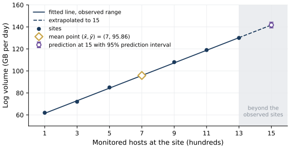
Figure 3.1. Least-squares line for the seven invented sites of the worked example, log volume in gigabytes (GB) per day against the number of monitored hosts in hundreds. The solid line is the fit \(\hat y = 55.7321 + 5.7321\,x\) of equation \eqref{eq:siteline} over the observed range of 1 to 13 hundred hosts. The dashed line extends it into the shaded region beyond the last site, up to the planned site with 1,500 hosts. The diamond marks the mean point \((\bar x, \bar y) = (7, 95.86)\), through which every least-squares line with an intercept passes. The open circle is the prediction of 141.71 GB per day at 15 hundred hosts, and its bar is the 95% prediction interval of equation \eqref{eq:predint}, from 139.19 to 144.24 GB per day, which is valid only if the straight line still holds there. Computed from equations \eqref{eq:simple} and \eqref{eq:predint}.
Show the answer
Without the column of ones, the normal equation has only the row \(\sum_i x_i(y_i - wx_i) = 0\), so \(w = \sum_i x_i y_i / \sum_i x_i^2\), which is \(5{,}339/455 \approx 11.734\). The residuals are 50.27, 36.80, 26.33, 12.86, 2.39, \(-10.07\) and \(-22.54\), which sum to about 96.03, not zero. Forced through the origin, the line is about twice as steep as the fit with an intercept. It underestimates the small sites, overestimates the large ones, and at \(x = 15\) predicts 176.01 GB per day instead of 141.71. Leaving out the intercept is justified only when the line must pass through the origin, and nothing requires that here.
Gradient descent
Gradient descent minimizes a differentiable loss by repeatedly stepping against its gradient,
where the learning rate \(\eta > 0\) sets the step size. For the four points of the first example, starting from \(\boldsymbol{\theta} = (0, 0)\), the gradient is \(-\frac{2}{4}X^\top\mathbf{y} = (-8, -23.5)\), and with \(\eta = 0.05\) the first step moves to \((b, w) = (0.4, 1.175)\). After two more steps the parameters are \((0.477, 1.401)\), already close to the solution \((0.5, 1.4)\) in the slope, while the intercept converges more slowly. Figure 3.2 shows gradient descent on the contours of the loss from another starting point, for a small learning rate and for one close to the stability limit.
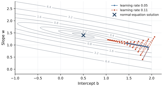
Figure 3.2. Gradient descent on the mean squared error of the four-point example. The contours are levels of the loss as a function of the intercept \(b\) and the slope \(w\); the cross marks the solution of the normal equation, \((0.5, 1.4)\). Both runs start at \((b, w) = (1.8, 0.4)\), a point chosen to make the geometry visible. With a learning rate of 0.05 (solid), the iterates drop quickly into the narrow valley and then creep along it toward the minimum. With a learning rate of 0.11 (dashed), close to the stability limit of about 0.12 for this loss, each step overshoots across the valley and the iterates zigzag, yet they advance further along it; above the limit they diverge. Neither run reaches the minimum within the 30 iterations shown. Computed from equation \eqref{eq:gd}.
When the loss is an average over \(n\) records, its gradient is an average of per-record gradients. Stochastic gradient descent (SGD) replaces the full average by the gradient on one randomly chosen record, or on a small random minibatch, at each step. Each step is noisy, but a step on one record costs \(n\) times less than a full-gradient step (a step on a minibatch of \(m\) records, \(n/m\) times less), and the noise averages out over many steps. Bottou (2010) argues that for large-scale problems, where computing time rather than the amount of data limits learning, SGD performs well, and shows that its averaged and second-order variants are asymptotically efficient after a single pass over the training set. Convergence results for plain SGD usually require that the learning rate \(\eta_t\) used at step \(t\) decrease over time, with \(\sum_t \eta_t = \infty\) and \(\sum_t \eta_t^2 < \infty\).
Gradient descent is one tool among several. Neural networks (Unit 5) are trained by variants of SGD because nothing else scales to their size. Scikit-learn's SGDClassifier trains linear models by SGD, which suits data that arrives as a stream. Many other models are fitted differently. LinearRegression solves a least-squares problem directly with a matrix decomposition. LogisticRegression uses L-BFGS by default, a quasi-Newton method that uses gradients but chooses its steps from an approximation to the curvature. Support vector machines solve a constrained quadratic program with a specialized solver. Decision trees are grown by a greedy search over splits, naive Bayes is fitted by counting or, in its Gaussian form, by computing a mean and a variance per class and feature, and k-nearest neighbors only stores the training data, at most organizing it in a search tree (a k-d tree or ball tree) for fast lookup. Gradient boosting uses gradients of the loss, but with respect to the model's predictions, and each of its trees is still grown greedily (Lesson 3.3).
Logistic regression
For a binary label \(y \in \{0, 1\}\), with 1 for attack, logistic regression models the probability of an attack as
where the sigmoid \(\sigma\) maps any real score \(z\) to \((0, 1)\). Inverting the sigmoid shows that the log-odds are linear in the features, \(\log\frac{p}{1-p} = \mathbf{w}^\top\mathbf{x} + b\). The decision boundary \(p = 0.5\) is the hyperplane \(\mathbf{w}^\top\mathbf{x} + b = 0\).
The parameters maximize the likelihood of the training labels, which is the same as minimizing the log-loss, also called the binary cross-entropy,
A confident wrong prediction is expensive. An attack scored \(p = 0.01\) costs \(-\log 0.01 = 4.6\), while one scored 0.5 costs 0.69 (Figure 3.3). Using \(\sigma'(z) = \sigma(z)(1 - \sigma(z))\), the gradient takes a simple form,
Each record adds its feature vector, weighted by its error \(p_i - y_i\), to the gradient, so a descent step moves the weights toward the features of an attack scored too low and away from the features of a normal record scored too high. The log-loss is convex in \((\mathbf{w}, b)\), so any local minimum is global, but unlike the MSE of linear regression it has no closed-form minimizer, and an iterative method is needed. If the training data can be separated perfectly by a hyperplane, the unpenalized log-loss keeps decreasing as \(\lVert\mathbf{w}\rVert\) grows, and the weights diverge; the penalties below prevent this.
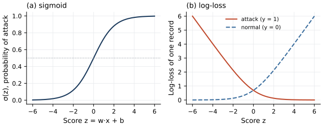
Figure 3.3. (a) The sigmoid function \(\sigma(z)\) of equation \eqref{eq:logistic}, mapping a linear score to a probability. (b) The log-loss of a single record as a function of the score \(z\), for an attack (\(y = 1\), red) and for a normal record (\(y = 0\), blue). The loss grows almost linearly for confident mistakes and approaches zero for confident correct predictions. Computed from equations \eqref{eq:logistic} and \eqref{eq:logloss}.
One gradient step by hand
Three records have one feature each, \(x = -1, 0, 2\), with labels \(y = 0, 0, 1\). Start from \(w = 0\) and \(b = 0\). Every prediction is \(\sigma(0) = 0.5\), and the loss is \(\log 2 \approx 0.693\). The errors \(p_i - y_i\) are 0.5, 0.5 and \(-0.5\). From \eqref{eq:loggrad},
and \(\partial L/\partial b\) is the mean error, \(\tfrac{1}{3}(0.5 + 0.5 - 0.5)\), which equals 0.1667. With \(\eta = 1\), the update \eqref{eq:gd} gives \(w = 0.5\) and \(b = -0.1667\). The new scores \(z = wx + b\) are \(-0.667\), \(-0.167\) and \(0.833\), so the predicted probabilities are 0.339, 0.458 and 0.697. The two normal records moved toward 0 and the attack toward 1, and the loss fell to
Show the answer
The gradient is the same, so \(w = 0 - 0.1 \times (-0.5)\), which is 0.05, and \(b = 0 - 0.1 \times 0.1667\), which is \(-0.0167\). A small enough step in the direction of the negative gradient always lowers a differentiable loss that is not already at a stationary point, because the first-order change in the loss is \(-\eta\lVert\nabla L\rVert^2 < 0\). The decrease is smaller than with \(\eta = 1\), so more steps are needed; too large a step can overshoot and raise the loss.
Regularization and the tradeoff between bias and variance
A model with many features can fit the training data closely by giving weight to accidents of the sample, such as a port that happened to appear in three attacks. Regularization adds a penalty on the size of the weights to the loss,
where \(\Omega(\mathbf{w}) = \lVert\mathbf{w}\rVert_2^2 = \sum_j w_j^2\) for the L2 penalty and \(\Omega(\mathbf{w}) = \lVert\mathbf{w}\rVert_1 = \sum_j |w_j|\) for the L1 penalty, \(\lambda \ge 0\) sets the strength, and the intercept is usually not penalized. The L2 penalty, which gives ridge regression in the linear case, shrinks all weights continuously toward zero. The L1 penalty, the lasso of Tibshirani (1996), tends to produce coefficients that are exactly zero, so it also selects features. Scikit-learn's LogisticRegression is parameterized by \(C\), which acts as an inverse penalty strength (it multiplies the summed data term instead of the penalty), so a small \(C\) means strong regularization. Because the penalty treats all weights alike, the features must be on comparable scales (Lesson 2.1).
The penalty trades two sources of error. For squared error, the expected error of a learned predictor \(\hat f\) at a point \(\mathbf{x}\), averaged over training sets and over the noise in \(y\), decomposes as
where \(f(\mathbf{x})\) is the true regression function and \(\sigma_\varepsilon^2\) the variance of the noise \(\varepsilon = y - f(\mathbf{x})\). The first term, the squared bias, measures how far the average learned model is from the truth; the second, the variance, measures how much the learned model changes from one training sample to another. Strong regularization lowers the variance and raises the bias, weak regularization does the opposite, and the best \(\lambda\) balances them. It is chosen on validation data or by cross-validation, never on the test set (Lesson 2.2).
Lab 3a fits L2- and L1-penalized logistic regressions over a range of \(C\) on the time-ordered split of the course data. Figure 3.4 shows the coefficients of the numeric features and the average precision (AP). With the L1 penalty at \(C = 0.001\), only 2 of the twelve numeric coefficients are nonzero, failed_logins and serror_rate, and the other numeric coefficients become nonzero as \(C\) grows. Test AP rises from 0.439 at the strongest L2 penalty to 0.522 at the weakest. With 26,275 training records and about two dozen feature columns, the variance of a linear model is small, and on this data a stronger penalty only adds bias. Lesson 3.3 shows the opposite case with decision trees.
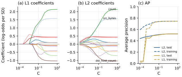
Figure 3.4. Regularization paths of logistic regression on the training days of Lab 3a. (a) and (b) Coefficients of the twelve standardized numeric features against \(C\) (logarithmic axis; small \(C\) means strong regularization) for the L1 and L2 penalties. The L1 path sets coefficients exactly to zero for small \(C\); the L2 path shrinks them smoothly. (c) Average precision on the training days (dashed) and on the test days (solid) for both penalties. Data from Lab 3a.
Show the answer
The data term cannot distinguish weight on one copy from weight on the other, since only the sum matters. The L2 penalty \(w_1^2 + w_2^2\) is smallest for a fixed sum when the weights are equal, so ridge spreads the effect evenly across the two. The L1 penalty \(|w_1| + |w_2|\) is the same for any split of a fixed sum with the same sign, so the lasso is indifferent and in practice tends to keep one and drop the other, with the choice sensitive to small changes in the data. Neither choice says which feature is the "real" cause.
Reading the coefficients
With standardized features, a coefficient \(w_j\) is the change in the log-odds of an attack for a one-standard-deviation increase in feature \(j\), holding the other features fixed, and \(e^{w_j}\) is the factor by which the odds are multiplied. In the logistic regression of Lab 3a (with the default \(C = 1\)), the coefficient of the log-transformed count is 1.85, that of the log-transformed srv_count is -0.43, and that of same_srv_rate is -0.53. Read one at a time, these say that more connections to a host raise the odds of an attack, while more connections to the same service, and a larger share of them, lower the odds. The three features measure overlapping things (same_srv_rate is roughly srv_count divided by count), so a connection cannot change one of them while the others stay fixed, and the model can trade weight between them. Their individual values, and even their signs, can change when one of the three is dropped or the regularization changes, while the combined effect on the score changes much less. The phrase "holding the other features fixed" describes a change that rarely happens in real traffic. Interpret coefficients as a group, and only after checking how correlated the features are.
Three further cautions apply in security. A coefficient describes association in the training data, not a causal mechanism. Coefficients change when the class balance or the regularization changes. And a linear detector whose weights are known tells an attacker which features to change. An attacker who can lower the features with positive weights, for example by spreading a scan over more time, lowers the score in a predictable way. Unit 7 studies such evasion attacks.
Probabilities from a logistic regression trained without reweighting are often close to calibrated on the training distribution, and are calibrated in large samples when the model is well specified. Niculescu-Mizil and Caruana (2005) found logistic regression well calibrated before any correction, and post-calibration did not help it on most of their eight test problems. With class_weight="balanced", the probabilities describe a world in which half of all records are attacks, and they must be corrected or recalibrated before being read as probabilities (Lesson 2.3).
Show the answer
The odds are \(0.2/0.8 = 0.25\). The coefficient multiplies them by \(e^{0.69} \approx 1.99\), giving odds of about 0.50 and a probability of \(0.50/1.50 \approx 0.33\). A coefficient acts on odds, so the change in probability depends on where you start; the same increase from \(p = 0.9\) would only reach about 0.95.
What the lab shows
Lab 3a
Comparing classifiers on a time-ordered split
Open in ColabRead with outputsNotebook on GitHubAbout 3 minutes to run on a laptop CPU
Lab 3a trains a logistic regression next to six other classifiers on the time-ordered split, computes the regularization paths shown in Figure 3.4 and prints the coefficients discussed above. Logistic regression is not the strongest model in that comparison, but it is fast, reproducible and easy to inspect, which is what a baseline should be.
Summary
Linear regression minimizes the mean squared error and has a closed-form solution, the normal equation, which is practical when the number of features is moderate. With one feature it reduces to the slope \(S_{xy}/S_{xx}\) and a line through the means, and a prediction outside the observed range of the feature is an extrapolation that the data cannot check. Logistic regression models the log-odds of an attack as a linear function of the features and minimizes the log-loss, whose gradient is the feature vector weighted by the prediction error; it has no closed form and is fitted iteratively. Gradient descent and its stochastic variants are the standard tools for large and streaming problems and for neural networks, while many other models are fitted by closed-form solutions, quasi-Newton methods, quadratic programming, greedy search or simple per-class statistics. L2 and L1 penalties trade variance for bias, with L1 also selecting features, and the penalty strength is a hyperparameter chosen on validation data. Coefficients on standardized features are changes in log-odds, but correlated features share their effect, and class weighting distorts the probabilities.
References
- Arp, D., Quiring, E., Pendlebury, F., Warnecke, A., Pierazzi, F., Wressnegger, C., Cavallaro, L., and Rieck, K. (2022). Dos and don'ts of machine learning in computer security. Proceedings of the 31st USENIX Security Symposium, 3971-3988. https://www.usenix.org/conference/usenixsecurity22/presentation/arp
- Bottou, L. (2010). Large-scale machine learning with stochastic gradient descent. Proceedings of COMPSTAT'2010, 177-186. https://doi.org/10.1007/978-3-7908-2604-3_16
- Niculescu-Mizil, A., and Caruana, R. (2005). Predicting good probabilities with supervised learning. Proceedings of the 22nd International Conference on Machine Learning, 625-632. https://doi.org/10.1145/1102351.1102430
- Tibshirani, R. (1996). Regression shrinkage and selection via the lasso. Journal of the Royal Statistical Society, Series B (Methodological), 58(1), 267-288. https://doi.org/10.1111/j.2517-6161.1996.tb02080.x