Unit 3 · Lesson 3.3
Decision trees, random forests and boosting
Decision trees split the feature space with a sequence of simple questions, such as whether the SYN-error rate exceeds 0.5 or whether more than three logins failed. One tree is easy to read and easy to overfit. Ensembles of trees, built by averaging many randomized trees (random forests) or by adding trees one at a time to reduce a loss (gradient boosting), are among the strongest general-purpose methods for tabular data such as flow records. This lesson builds a split by hand, explains why averaging and boosting work, compares the classifiers of the unit on the course data, and separates global feature importance from the explanation of a single alert.
Growing a decision tree
A classification tree partitions the feature space into rectangular regions by recursive binary splits of the form \(x_j \le t\). It is grown greedily. At each node, every candidate feature \(j\) and threshold \(t\) is tried, the one that makes the two child nodes purest is kept, and the procedure repeats in each child until a stopping rule applies (a maximum depth, a minimum number of records per leaf, or a pure node). A leaf predicts the share of attacks among the training records that reach it.
Purity is measured by an impurity function of the class shares in a node. For a node in which a share \(p\) of the records are attacks, the Gini impurity, \(1 - p^2 - (1-p)^2\), and the entropy are
Both are zero for a pure node and largest at \(p = 0.5\). A split of a node with \(n\) records into children with \(n_L\) and \(n_R\) records is scored by the decrease in impurity,
where \(I\) is \(G\) or \(H\). With entropy, \(\Delta\) is the information gain used by Quinlan (1986) in the ID3 algorithm.
The features of flows.csv follow the KDD Cup 1999 intrusion data, which combines basic features of a connection, traffic features over recent connections to the same host or service (such as count and serror_rate), and content features such as failed logins (Tavallaee et al., 2009). Consider a node with 100 connections, 20 of them attacks. Two candidate splits are serror_rate > 0.5, which sends 25 records (17 attacks) to the right and 75 (3 attacks) to the left, and count > 40, which sends 30 records (16 attacks) to the right and 70 (4 attacks) to the left. The table below gives the share of attacks, Gini impurity and entropy of each node.
| Node | Records (attacks) | Attack share | Gini | Entropy (bits) |
|---|---|---|---|---|
| Parent | 100 (20) | 0.200 | 0.320 | 0.722 |
| serror_rate ≤ 0.5 | 75 (3) | 0.040 | 0.077 | 0.242 |
| serror_rate > 0.5 | 25 (17) | 0.680 | 0.435 | 0.904 |
| count ≤ 40 | 70 (4) | 0.057 | 0.108 | 0.316 |
| count > 40 | 30 (16) | 0.533 | 0.498 | 0.997 |
From the table, the split on serror_rate leaves a weighted Gini impurity of \(0.75 \times 0.0768\) plus \(0.25 \times 0.4352\), or 0.166, a decrease of 0.154, and a weighted entropy of 0.408, an information gain of 0.314 bits. The split on count leaves 0.225 (a decrease of 0.095) and 0.520 bits (a gain of 0.202 bits). Both criteria prefer the split on serror_rate. Figure 3.9 draws the chosen split.
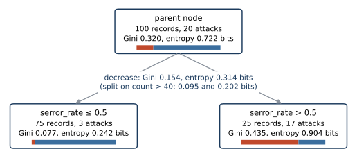
Figure 3.9. The worked split of the text. A node of 100 connections (20 attacks) is split on serror_rate at 0.5. Bars inside each node show the share of attacks (red) and normal connections (blue); the numbers give the records, attacks, Gini impurity and entropy of each node. The impurity decreases of equation \eqref{eq:gain} for this split and for the competing split on count are printed between the levels. Schematic of a hand computation.
A split depends only on the order of a feature's values, so trees need no scaling or log transforms (Lesson 2.1). Trees handle mixtures of numeric and categorical features and capture interactions, since a split on one feature is followed by different splits in each branch. They are also unstable, because a small change in the training data can change the top split and with it the entire tree.
Depth and overfitting
A tree grown until every leaf is pure fits the training data perfectly and generalizes poorly. Lab 3a grows trees of increasing depth on the training days of the course data (Figure 3.10). A tree of depth 1 reaches a test AP of 0.247, which is underfitting. Test AP peaks at 0.520 at depth 6, and a fully grown tree reaches a training AP of 1.00 and a test AP of 0.458. Depth, the minimum number of records per leaf, and cost-complexity pruning (ccp_alpha in scikit-learn) all limit this growth. They are hyperparameters to be chosen on validation data, never on the test curve shown here (Lesson 2.2).
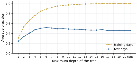
Figure 3.10. Average precision of a single decision tree on the training days (dashed) and the test days (solid) of Lab 3a, as a function of its maximum depth; "none" is a tree grown until its leaves are pure. Training AP keeps rising with depth, while test AP rises, peaks and declines, the signature of underfitting followed by overfitting. Data from Lab 3a.
Bagging and random forests
Bagging, introduced by Breiman (1996), trains each model on a bootstrap sample, \(n\) records drawn with replacement from the \(n\) training records, and aggregates the models. Breiman identified the instability of the base procedure as the vital element; aggregation helps when perturbing the training set changes the predictor a lot. A given record is left out of a bootstrap sample with probability \((1 - 1/n)^n\), which approaches \(e^{-1} \approx 0.368\) as \(n\) grows, so each tree sees about 63% of the distinct records, and the rest serve as out-of-bag test data for that tree.
Averaging helps because it cancels the part of the trees' errors that they do not share. Let the predictions of \(B\) trees at a point be random variables with common variance \(\sigma^2\) and pairwise correlation \(\rho\). The variance of their average is
which follows from summing the \(B\) variances and the \(B(B-1)\) covariances \(\rho\sigma^2\) and dividing by \(B^2\). The second term vanishes as \(B\) grows, but the first does not. With \(\rho = 0.3\) and \(B = 300\), the variance falls to \(0.3 + 0.7/300 \approx 0.302\) times that of one tree. Averaging removes neither the shared part of the error nor any bias; if every tree misses the same attacks, so does the forest.
Random forests reduce the first term by decorrelating the trees. Breiman (2001) grew each tree on a bootstrap sample and, at each node, searched for the best split only among a small random subset of the features. He showed that the generalization error of a forest converges as trees are added, so adding trees does not cause overfitting, and that its accuracy depends on the strength of the individual trees and the correlation between them. In scikit-learn, max_features sets the size of the random subset (by default the square root of the number of features for classification), and the forest's probability is the average of the trees' leaf probabilities, a choice that differs from Breiman's majority vote. A forest of fully grown trees fits its training data almost perfectly and still predicts new data well, because the errors of its trees are partly independent and cancel in the average.
Show the answer
With \(B = 500\) the variance is \(\sigma^2(0.5 + 0.5/500)\), or \(0.501\,\sigma^2\); with \(B = 1{,}000\) it is \(0.5005\,\sigma^2\), a reduction of about 0.1%. Once \(B\) is large, the correlation term dominates. Decorrelating the trees, for example by considering fewer features at each split, reduces \(\rho\) and so the floor of the variance, although each tree becomes somewhat weaker; the best tradeoff is found on validation data.
Gradient boosting
Boosting builds an additive model in stages. Friedman (2001) viewed this as gradient descent in the space of functions. Let \(F_{m-1}(\mathbf{x})\) be the ensemble after \(m - 1\) stages, a score whose sigmoid is the predicted probability of attack, and \(L(y, F)\) a differentiable loss. Stage \(m\) computes, for every training record, the negative gradient of the loss with respect to the ensemble's current output,
fits a regression tree \(T_m\) to these pseudo-residuals by least squares, sets the value of each leaf by a line search on the loss, and adds the tree with a learning rate \(\eta\) (Friedman's shrinkage), \(F_m = F_{m-1} + \eta\,T_m\). For the log-loss of Lesson 3.1 with labels \(y \in \{0, 1\}\), the pseudo-residual is \(r_{im} = y_i - p_{i,m-1}\), the gap between the label and the current ensemble's probability, and Friedman approximated the line search in each leaf by a single Newton step, which uses the second derivative of the loss. Each new tree targets the errors of the whole ensemble so far, in proportion to their size. In Friedman's simulations, smaller learning rates gave better performance, with diminishing returns, at the cost of more stages, while large rates overfit as stages were added. The number of stages is therefore chosen by early stopping, which stops adding stages once the loss on validation data no longer improves.
The XGBoost system of Chen and Guestrin (2016) builds the second derivative into the objective itself. It minimizes a regularized objective with a penalty on the number of leaves and on the leaf values, and a second-order expansion of the loss gives both a score for candidate splits and the optimal value of leaf \(\ell\),
where \(R_\ell\) is the set of training records in leaf \(\ell\), \(g_i\) and \(h_i\) are the first and second derivatives of the loss for record \(i\) with respect to \(F\), at \(F = F_{m-1}(\mathbf{x}_i)\), and \(\lambda\) is the L2 penalty on leaf values. With \(\lambda = 0\) this is the Newton step of Friedman's algorithm. Scikit-learn's HistGradientBoostingClassifier computes leaf values with the same formula.
A worked stage makes this concrete. Take the node of the tree example, 100 records with 20 attacks, as the whole training set. The initial model is the constant log-odds \(F_0 = \log(0.2/0.8) = -1.386\), so every record has \(p = 0.2\). For the log-loss, \(g_i = p_i - y_i\) and \(h_i = p_i(1 - p_i) = 0.16\). Fit a one-split tree on serror_rate. The left leaf holds 75 records with 3 attacks, so \(\sum g_i\) is \(72 \times 0.2 - 3 \times 0.8\), or 12, and \(\sum h_i = 75 \times 0.16 = 12\), giving \(w^* = -1.0\) with \(\lambda = 0\). The right leaf holds 25 records with 17 attacks, so \(\sum g_i\) is \(8 \times 0.2 - 17 \times 0.8\), or \(-12\), and \(\sum h_i = 4\), giving \(w^* = 3.0\). With \(\eta = 0.1\), the left records move to \(F_1 = -1.486\) (\(p = 0.184\)) and the right records to \(F_1 = -1.086\) (\(p = 0.252\)).
XGBoost also learns a default direction for missing values at each split and offers an approximate split search based on weighted quantiles. LightGBM (Ke et al., 2017) buckets continuous feature values into discrete bins, searches splits over the bins, samples records by gradient size and bundles mutually exclusive features; its authors report training up to over 20 times faster than conventional gradient boosting with almost the same accuracy. Scikit-learn's HistGradientBoostingClassifier is a histogram-based implementation inspired by LightGBM. It handles missing values natively and by default stops early on an internal validation split when the training set has more than 10,000 records, as in Lab 3a.
Why tree ensembles do well on tabular data
Grinsztajn et al. (2022) benchmarked tree-based models against deep learning architectures on 45 tabular datasets from varied domains. They kept independent and identically distributed data (stream-like datasets and time series were removed), truncated training sets to 10,000 samples, removed missing data, and reduced classification targets to two balanced classes. Tree-based models remained the state of the art on these medium-sized datasets, even without accounting for their speed. The authors attribute the gap to inductive biases. Trees are robust to uninformative features, respect the orientation of the data (each split uses one original feature), and can learn irregular functions. Flow records with a few dozen numeric and categorical features resemble the benchmark datasets, but security data adds heavy class imbalance, drift and adversaries, none of which the benchmark measures.
Comparing the classifiers of the unit
Lab 3a trains seven classifiers on the time-ordered split of the course data, with five seeds for the models that have a random component, and computes a bootstrap interval for AP over test records. Figure 3.11 and the table below summarize the results.
| Classifier | AP, mean ± sd over seeds | AP, 95% bootstrap interval | Recall at 100 alerts per day |
|---|---|---|---|
| Logistic regression | 0.518 ± 0.000 | 0.468 to 0.561 | 0.486 |
| k-nearest neighbors (k = 25) | 0.571 ± 0.000 | 0.524 to 0.614 | 0.563 |
| SVM, RBF kernel | 0.613 ± 0.000 | 0.569 to 0.656 | 0.583 |
| Gaussian naive Bayes | 0.310 ± 0.000 | 0.268 to 0.351 | 0.461 |
| Decision tree (depth 8) | 0.500 ± 0.003 | 0.451 to 0.545 | 0.506 |
| Random forest (300 trees) | 0.701 ± 0.010 | 0.653 to 0.732 | 0.606 |
| Histogram gradient boosting | 0.654 ± 0.017 | 0.612 to 0.691 | 0.569 |
The standard deviation over seeds measures only training randomness and is zero for the deterministic models. The bootstrap interval, computed for the model trained with the first seed, resamples test records and reflects the size of the test set; records of one host and day are not independent, so the true uncertainty is larger. Recall within the budget is the expected value when records tied at the cutoff are alerted in random order. The random forest has the highest AP, but its interval overlaps that of gradient boosting, used here with default settings and no tuning, so the order of the two is not secure. Gaussian naive Bayes is clearly the weakest, and the remaining models lie in between, with overlapping intervals for neighbors in the ranking. At 20 alerts per day the budget is too small to separate the models, since recall cannot exceed 0.185 even when every alert is a real attack, so the table reports a budget of 100 alerts per day instead.
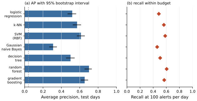
Figure 3.11. Average precision on the test days of Lab 3a for the seven classifiers of the unit (bars, mean over five seeds where applicable), with 95% bootstrap intervals over test records for the model trained with the first seed (black lines), and recall within a budget of 100 alerts per day (diamonds, right panel). The dotted line in the left panel is the base rate of the test days. Data from Lab 3a.
The per-family recall at the same budget in the table below, averaged over seeds, shows where the remaining errors are.
| Classifier | scan | brute-force | dos | exfil | c2beacon |
|---|---|---|---|---|---|
| Logistic regression | 0.92 | 0.78 | 0.96 | 0.52 | 0.01 |
| k-nearest neighbors | 1.00 | 0.93 | 1.00 | 0.91 | 0.00 |
| SVM, RBF kernel | 0.99 | 0.95 | 0.98 | 0.94 | 0.04 |
| Gaussian naive Bayes | 0.91 | 0.73 | 1.00 | 0.30 | 0.00 |
| Decision tree | 0.87 | 0.87 | 0.95 | 0.76 | 0.00 |
| Random forest | 1.00 | 0.96 | 0.98 | 0.96 | 0.08 |
| Gradient boosting | 0.99 | 0.96 | 1.00 | 0.95 | 0.00 |
Every classifier catches most scanning, brute-force and denial-of-service records, and almost none of the 180 command-and-control beacons, which never occur in the training days. Record by record, a beacon looks like ordinary web traffic, and no classifier learns a family that is absent from its training data. Detecting beaconing needs different features, such as the regularity of a host's connections over hours, and, for a supervised classifier, labeled examples of the family. On this data the features and the coverage of the labels matter more than the choice of model.
What the model learned
Tree ensembles offer two global measures of feature importance. Impurity importance, called Gini importance by Strobl et al. (2007), adds up, for each feature, the impurity decrease of every split that uses it, weighted by the share of records reaching the split, and averages over trees. It is computed on the training data and is biased. Strobl and colleagues showed in simulations that random forest importance measures are unreliable when the features vary in their scale of measurement or their number of categories, with the Gini importance most strongly biased, because a feature with many possible split points is more likely to produce a good split by chance, as in multiple testing.
Permutation importance, which Breiman (2001) used to measure variable importance in random forests, permutes the values of one feature in held-out data, breaking its link to the label while keeping its distribution, and measures how much a performance metric drops. In the simulations of Strobl and colleagues its average for an uninformative feature was close to zero, but its spread grew with the number of categories, so a single run can still overstate or understate a feature. Lab 3a adds a column of pure noise to the training and test data of a random forest. Its impurity importance is 0.0160, ranked 14 of 25 columns and above most of the one-hot indicator columns of the categorical features, while its permutation importance on the test days is 0.0003. For the random forest, the model with the highest mean AP, the permutation importances in AP are largest for service (0.176) and dst_host_count (0.095), as Figure 3.12 shows. When two features are strongly correlated, permuting one leaves the other to carry the information, so both can look unimportant, and permuting creates combinations of values that never occur in real traffic.
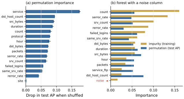
Figure 3.12. (a) Permutation importance of each original feature for the random forest of Lab 3a, measured as the drop in test AP when the feature is shuffled (mean over five repetitions, bars; one standard deviation, lines). One-hot columns of a categorical feature are shuffled together. (b) Impurity importance (share of the total impurity decrease on the training data) and permutation importance (drop in test AP) of a forest trained with an added column of random noise, for the fourteen columns with the largest impurity importance. The noise column (highlighted) receives impurity importance comparable to that of several real columns but almost no permutation importance. Data from Lab 3a.
Explaining one alert
Both importances describe the model as a whole. An analyst triaging an alert needs to know why one particular connection was flagged, and a feature can be globally important and irrelevant for that alert, or globally minor and decisive for it.
Local explanations attribute a single prediction to the features. Lundberg and Lee (2017) consider additive feature attributions, which explain a prediction \(f(\mathbf{x})\) as a base value plus one contribution \(\phi_j\) per feature, and show that only one such attribution satisfies three properties, namely local accuracy (the contributions sum to the prediction minus the base value), missingness (a feature missing from the input receives no contribution) and consistency (if the model changes so that revealing a feature adds at least as much to the output as before, whatever other features are known, that feature's contribution does not decrease). It is given by the Shapley values of cooperative game theory, which they call SHAP values when the game is defined by conditional expectations of the model's output. For a feature \(j\) in the set \(\mathcal{F}\) of all features,
where \(f_S(\mathbf{x})\) is the model's output when only the features in \(S\) are known. Equivalently, \(\phi_j\) is the average, over all orders in which the features could be revealed, of the change in output when feature \(j\) is revealed.
Here is a toy example. A detector's score for a connection is 0 when no features are known (the base value), 0.5 when only its failed-login count is known, 0.3 when only its connection count is known, and 1.0 when both are known; a third feature, the hour, changes nothing. Over the six orders of revealing the three features, failed logins adds 0.5 when revealed before count and 0.7 when revealed after it, so \(\phi_{\text{logins}} = (0.5 + 0.7)/2\), which is 0.6. Count adds 0.3 or 0.5, so \(\phi_{\text{count}} = 0.4\), and \(\phi_{\text{hour}} = 0\). The contributions sum to \(1.0\), the prediction minus the base value. The interaction between the two features, the extra 0.2 that appears only when both are known, is split equally between them.
SHAP values describe the model. They show what it relied on for this alert, which can reveal a shortcut (a template artifact, a leaked column) as well as a genuine indicator. Exact computation over all subsets is exponential in the number of features, so practical tools approximate it or use algorithms specific to a model class, and their results depend on how "unknown" features are filled in. An explanation shown to analysts is also information shown to anyone who can see it, and an attacker who learns which features drive a detector learns what to change.
Show the answer
Failed logins now adds 0.5 when revealed before count and 1.1 when revealed after it, so \(\phi_{\text{logins}} = 0.8\); count adds 0.3 or 0.9, so \(\phi_{\text{count}} = 0.6\). They sum to 1.4, the new prediction minus the base value, which is local accuracy. Both contributions rose because each feature's marginal effect rose or stayed the same in every context, which is the consistency property. A feature whose marginal effect never decreases, in any context, cannot receive a smaller contribution.
What the lab shows
Lab 3a
Comparing classifiers on a time-ordered split
Open in ColabRead with outputsNotebook on GitHubAbout 3 minutes to run on a laptop CPU
Lab 3a runs the comparison of this lesson, the depth sweep and the importance analysis. Try changing max_features of the random forest and watch how its AP and the spread over seeds respond.
Summary
A decision tree chooses each split greedily to maximize the decrease in Gini impurity or entropy, needs no scaling, captures interactions, and overfits as it grows deeper. Bagging averages trees trained on bootstrap samples and helps because trees are unstable; random forests also restrict each split to a random subset of features, which lowers the correlation between trees that averaging cannot remove. Gradient boosting adds trees fitted to the negative gradient of the loss of the whole ensemble, with shrinkage and Newton-step leaf values, and XGBoost adds a regularized second-order objective for choosing splits. Tree ensembles are strong on medium-sized tabular data, but no classifier detects a family absent from training. Impurity importance favors features with many split points, permutation importance on held-out data is more reliable, and only local attributions such as SHAP values explain an individual alert.
References
- Breiman, L. (1996). Bagging predictors. Machine Learning, 24(2), 123-140. https://doi.org/10.1007/BF00058655
- Breiman, L. (2001). Random forests. Machine Learning, 45(1), 5-32. https://doi.org/10.1023/A:1010933404324
- Chen, T., and Guestrin, C. (2016). XGBoost: A scalable tree boosting system. Proceedings of the 22nd ACM SIGKDD International Conference on Knowledge Discovery and Data Mining, 785-794. https://doi.org/10.1145/2939672.2939785
- Friedman, J. H. (2001). Greedy function approximation: A gradient boosting machine. The Annals of Statistics, 29(5), 1189-1232. https://doi.org/10.1214/aos/1013203451
- Grinsztajn, L., Oyallon, E., and Varoquaux, G. (2022). Why do tree-based models still outperform deep learning on typical tabular data?. Advances in Neural Information Processing Systems 35, Datasets and Benchmarks Track, 507-520. https://doi.org/10.52202/068431-0037
- Ke, G., Meng, Q., Finley, T., Wang, T., Chen, W., Ma, W., Ye, Q., and Liu, T.-Y. (2017). LightGBM: A highly efficient gradient boosting decision tree. Advances in Neural Information Processing Systems 30. https://proceedings.neurips.cc/paper_files/paper/2017/hash/6449f44a102fde848669bdd9eb6b76fa-Abstract.html
- Lundberg, S. M., and Lee, S.-I. (2017). A unified approach to interpreting model predictions. Advances in Neural Information Processing Systems 30. https://proceedings.neurips.cc/paper_files/paper/2017/hash/8a20a8621978632d76c43dfd28b67767-Abstract.html
- Quinlan, J. R. (1986). Induction of decision trees. Machine Learning, 1(1), 81-106. https://doi.org/10.1007/BF00116251
- Strobl, C., Boulesteix, A.-L., Zeileis, A., and Hothorn, T. (2007). Bias in random forest variable importance measures: Illustrations, sources and a solution. BMC Bioinformatics, 8, 25. https://doi.org/10.1186/1471-2105-8-25
- Tavallaee, M., Bagheri, E., Lu, W., and Ghorbani, A. A. (2009). A detailed analysis of the KDD CUP 99 data set. 2009 IEEE Symposium on Computational Intelligence for Security and Defense Applications, 1-6. https://doi.org/10.1109/CISDA.2009.5356528