Unit 3 · Lab 3a
Comparing classifiers on a time-ordered split
Lab 3a
Comparing classifiers on a time-ordered split
Open in ColabRead with outputsNotebook on GitHubAbout 3 minutes to run on a laptop CPU
# On Google Colab, install the scikit-learn version the course was built with.
# On your own computer, install requirements.txt instead; this cell then does nothing.
import subprocess, sys
if "google.colab" in sys.modules:
    subprocess.run([sys.executable, "-m", "pip", "install", "-q", "scikit-learn==1.9.0"], check=True)
Lab 3a. Comparing classifiers on a time-ordered split
This lab trains the supervised models of Unit 3 on the same data and the same time-ordered split, and compares them the way a security team would, by average precision (AP), by the share of attacks caught within an alert budget, and by attack family. It then looks inside the highest-scoring model with permutation importance and shows over- and underfitting by varying the depth of a decision tree. It runs in a few minutes on a laptop CPU.
You will:
- prepare the features once, fitting every preprocessing step on the training days only;
- train seven classifiers and compare them over five seeds;
- measure recall per attack family within an alert budget;
- compute permutation importance for the model with the highest AP, and compare it with impurity importance;
- sweep the depth of a decision tree and the regularization strength of a logistic regression;
- draw the decision boundaries of four models on two features.
The data is synthetic (Lesson 1.3). Training uses days 0 to 9 and testing days 10 to 13, after removing duplicated records (Lesson 2.2).
import os
import time
import warnings

import numpy as np
import pandas as pd
import matplotlib.pyplot as plt

from sklearn.compose import ColumnTransformer
from sklearn.ensemble import HistGradientBoostingClassifier, RandomForestClassifier
from sklearn.inspection import permutation_importance
from sklearn.linear_model import LogisticRegression
from sklearn.metrics import average_precision_score
from sklearn.naive_bayes import GaussianNB
from sklearn.neighbors import KNeighborsClassifier
from sklearn.pipeline import make_pipeline
from sklearn.preprocessing import FunctionTransformer, OneHotEncoder, StandardScaler
from sklearn.svm import SVC
from sklearn.tree import DecisionTreeClassifier

warnings.filterwarnings("ignore")

LOCAL = "../../data/flows.csv"
URL = "https://raw.githubusercontent.com/aalbata/machine-learning-for-cybersecurity/main/data/flows.csv"
flows = pd.read_csv(LOCAL if os.path.exists(LOCAL) else URL).drop_duplicates().reset_index(drop=True)
train = flows[flows["day"] <= 9]
test = flows[flows["day"] >= 10]
ytr = train["label"].to_numpy()
yte = test["label"].to_numpy()
family = test["attack_type"].to_numpy()
SEEDS = [0, 1, 2, 3, 4]
print(f"training records {len(train):,} ({ytr.sum()} attacks), test records {len(test):,} ({yte.sum()} attacks)")
print(test["attack_type"].value_counts().to_dict())
training records 26,275 (608 attacks), test records 10,495 (432 attacks)
{'normal': 10063, 'c2beacon': 180, 'scan': 86, 'bruteforce': 83, 'dos': 50, 'exfil': 33}
1. Features
The skewed duration, byte, packet and connection-count columns (duration, src_bytes, dst_bytes, packets, count, srv_count) are log-transformed, every numeric column is standardized, and the categorical columns are one-hot encoded. The scaling matters for logistic regression, k-nearest neighbors and the support vector machine; it is harmless for the tree models, whose splits depend only on the order of the values.
skewed = ["duration", "src_bytes", "dst_bytes", "packets", "count", "srv_count"]
plain = ["failed_logins", "serror_rate", "rerror_rate", "same_srv_rate", "dst_host_count", "hour"]
categorical = ["protocol", "service", "site"]
prep = ColumnTransformer([
    ("log", make_pipeline(FunctionTransformer(np.log1p, feature_names_out="one-to-one"), StandardScaler()), skewed),
    ("num", StandardScaler(), plain),
    ("cat", OneHotEncoder(handle_unknown="ignore", sparse_output=False), categorical),
]).fit(train)
Xtr = prep.transform(train)
Xte = prep.transform(test)
feature_names = [n.split("__", 1)[1] for n in prep.get_feature_names_out()]
print(Xtr.shape, Xte.shape)
(26275, 24) (10495, 24)
2. Seven classifiers
Each model outputs a score for every test record; for the support vector machine the score is the value of its decision function, which is proportional to the signed distance from the separating hyperplane in the kernel's feature space, and for the others it is a predicted probability. AP and recall within a budget depend only on the ranking, so the two kinds of score can be compared. Models with a random component (the decision tree's tie-breaking, the forest's bootstrap samples and feature subsets, gradient boosting's early-stopping split) are trained with five seeds. The others are deterministic, so their standard deviation is zero.
The alert budget is expressed per day. At 20 alerts per day (80 over the four test days), almost every model fills the budget with real attacks, so recall is capped at 80 divided by the number of test attacks and says little about the differences between models. We therefore also report recall at 100 alerts per day.
Several models give many records exactly the same score (a k-NN score is a multiple of 1/25, a tree gives every record in a leaf the same probability, and naive Bayes gives many records a probability that is exactly 1 in floating point). When the records tied at the cutoff do not all fit in the budget, which of them are alerted is arbitrary. The function recall_at therefore reports the expected recall when ties are broken at random, counting each tied record as a fraction of an alert.
def make(name, seed):
    return {
        "logistic regression": LogisticRegression(max_iter=10000, tol=1e-8),
        "k-nearest neighbors": KNeighborsClassifier(n_neighbors=25),
        "SVM (RBF kernel)": SVC(kernel="rbf", C=1.0, gamma="scale"),
        "Gaussian naive Bayes": GaussianNB(),
        "decision tree": DecisionTreeClassifier(max_depth=8, random_state=seed),
        "random forest": RandomForestClassifier(n_estimators=300, n_jobs=-1, random_state=seed),
        "gradient boosting": HistGradientBoostingClassifier(random_state=seed),
    }[name]


RANDOM = {"decision tree", "random forest", "gradient boosting"}
NAMES = ["logistic regression", "k-nearest neighbors", "SVM (RBF kernel)", "Gaussian naive Bayes",
         "decision tree", "random forest", "gradient boosting"]
n_days = test["day"].nunique()


def score_of(model, X):
    return model.predict_proba(X)[:, 1] if hasattr(model, "predict_proba") else model.decision_function(X)


def recall_at(score, k):
    """Expected recall when the k highest-scoring records are alerted and ties at the cutoff are broken at random."""
    cutoff = np.sort(score)[::-1][k - 1]
    above = score > cutoff
    tied = score == cutoff
    alert = above.astype(float)
    alert[tied] = (k - above.sum()) / tied.sum()
    return alert[yte == 1].mean(), alert


rows, scores0, seconds = [], {}, {}
for name in NAMES:
    t0 = time.time()
    for s in (SEEDS if name in RANDOM else [0]):
        model = make(name, s).fit(Xtr, ytr)
        sc = score_of(model, Xte)
        r20, _ = recall_at(sc, 20 * n_days)
        r100, alert = recall_at(sc, 100 * n_days)
        rows.append(dict(model=name, seed=s, ap=average_precision_score(yte, sc), recall20=r20, recall100=r100,
                         **{f"fam_{f}": alert[family == f].mean() for f in ["scan", "bruteforce", "dos", "exfil", "c2beacon"]}))
        if s == 0:
            scores0[name] = sc
            if name == "random forest":
                rf0 = model
    seconds[name] = time.time() - t0
runs = pd.DataFrame(rows)
table = runs.groupby("model", sort=False).agg(ap=("ap", "mean"), ap_sd=("ap", "std"),
                                              recall20=("recall20", "mean"),
                                              recall100=("recall100", "mean"), recall100_sd=("recall100", "std")).fillna(0.0)
table["seconds"] = pd.Series(seconds)
print(table.round(3).to_string())
print(f"ceiling on recall at 20 alerts per day: {20 * n_days / yte.sum():.3f}")
ap ap_sd recall20 recall100 recall100_sd seconds model logistic regression 0.518 0.000 0.185 0.486 0.000 0.614 k-nearest neighbors 0.571 0.000 0.185 0.563 0.000 0.467 SVM (RBF kernel) 0.613 0.000 0.185 0.583 0.000 1.218 Gaussian naive Bayes 0.310 0.000 0.093 0.461 0.000 0.027 decision tree 0.500 0.003 0.177 0.506 0.004 0.757 random forest 0.701 0.010 0.185 0.606 0.003 6.864 gradient boosting 0.654 0.017 0.185 0.569 0.002 2.861 ceiling on recall at 20 alerts per day: 0.185
The standard deviation over seeds measures only the randomness inside training. It says nothing about how much the scores would change on other test days. A rough view of that second source of uncertainty is a bootstrap over test records, which resamples the test set with replacement many times and recomputes AP. Records from the same host and day are not independent, so the interval below is too narrow, but it shows which differences are large compared with the sampling noise. The bootstrap uses the models trained with the first seed, so for the three models with a random component the AP printed below differs slightly from the mean over seeds in the table above.
rng = np.random.default_rng(0)
boot_idx = [rng.integers(0, len(yte), len(yte)) for _ in range(200)]
boot = {}
for name, sc in scores0.items():
    vals = [average_precision_score(yte[i], sc[i]) for i in boot_idx]
    boot[name] = (float(np.percentile(vals, 2.5)), float(np.percentile(vals, 97.5)))
    print(f"{name:<22} AP {average_precision_score(yte, sc):.3f}  bootstrap 95% interval {boot[name][0]:.3f} to {boot[name][1]:.3f}")
logistic regression AP 0.518 bootstrap 95% interval 0.468 to 0.561
k-nearest neighbors AP 0.571 bootstrap 95% interval 0.524 to 0.614
SVM (RBF kernel) AP 0.613 bootstrap 95% interval 0.569 to 0.656
Gaussian naive Bayes AP 0.310 bootstrap 95% interval 0.268 to 0.351
decision tree AP 0.495 bootstrap 95% interval 0.451 to 0.545
random forest AP 0.694 bootstrap 95% interval 0.653 to 0.732
gradient boosting AP 0.653 bootstrap 95% interval 0.612 to 0.691
3. Recall by attack family
The table gives the share of each family's test records that fall inside the budget of 100 alerts per day, averaged over seeds. The c2beacon family never occurs in the training days.
fam_table = runs.groupby("model", sort=False)[[c for c in runs.columns if c.startswith("fam_")]].mean()
fam_table.columns = [c[4:] for c in fam_table.columns]
print(fam_table.round(2).to_string())
scan bruteforce dos exfil c2beacon model logistic regression 0.92 0.78 0.96 0.52 0.01 k-nearest neighbors 1.00 0.93 1.00 0.91 0.00 SVM (RBF kernel) 0.99 0.95 0.98 0.94 0.04 Gaussian naive Bayes 0.91 0.73 1.00 0.30 0.00 decision tree 0.87 0.87 0.95 0.76 0.00 random forest 1.00 0.96 0.98 0.96 0.08 gradient boosting 0.99 0.96 1.00 0.95 0.00
Every model catches most scans, brute-force attempts and denial-of-service records within the budget, and almost no command-and-control beacons. No choice of classifier repairs a gap in the training data. The beacons resemble ordinary web traffic in each single record, and detecting them needs features that describe a host's behavior over time, such as the regularity of its connections.
4. What does the highest-scoring model rely on?
The model with the highest mean AP is examined next. Its bootstrap interval in the printout above overlaps that of the model with the second-highest mean AP, so the order of the two is not secure. Permutation importance shuffles one column of the test data at a time and measures how much AP drops. The shuffle breaks the link between that column and the label while keeping its distribution. One-hot columns of the same categorical feature are shuffled together, by permuting the original column before preprocessing.
best = table["ap"].idxmax()
print("highest mean AP:", best)
raw_cols = skewed + plain + categorical
best_pipe = make_pipeline(prep, make(best, 0)).fit(train, ytr)
pi = permutation_importance(best_pipe, test[raw_cols], yte, scoring="average_precision", n_repeats=5,
                            random_state=0)
perm = pd.DataFrame({"mean": pi.importances_mean, "sd": pi.importances_std}, index=raw_cols).sort_values("mean", ascending=False)
print(perm.round(4).to_string())
highest mean AP: random forest
                  mean      sd
service         0.1758  0.0030
dst_host_count  0.0948  0.0006
src_bytes       0.0913  0.0026
duration        0.0876  0.0032
count           0.0809  0.0037
protocol        0.0788  0.0023
hour            0.0764  0.0050
dst_bytes       0.0731  0.0018
packets         0.0712  0.0019
serror_rate     0.0685  0.0029
srv_count       0.0660  0.0042
failed_logins   0.0567  0.0009
same_srv_rate   0.0534  0.0014
rerror_rate     0.0421  0.0020
site            0.0015  0.0009
A random forest also reports impurity importance, the total decrease in Gini impurity produced by splits on each feature, averaged over trees. It is computed on the training data and is known to favor features with many distinct values. To see this, we add a column of pure noise to the training and test data, train the forest again, and compare both importances for the noise column.
noise_rng = np.random.default_rng(1)
Xtr_n = np.hstack([Xtr, noise_rng.normal(size=(len(Xtr), 1))])
Xte_n = np.hstack([Xte, noise_rng.normal(size=(len(Xte), 1))])
names_n = feature_names + ["noise"]
rf_noise = RandomForestClassifier(n_estimators=300, n_jobs=-1, random_state=0).fit(Xtr_n, ytr)
imp_impurity = pd.Series(rf_noise.feature_importances_, index=names_n)
pi_n = permutation_importance(rf_noise, Xte_n, yte, scoring="average_precision", n_repeats=5, random_state=0)
imp_perm = pd.Series(pi_n.importances_mean, index=names_n)
compare = pd.DataFrame({"impurity": imp_impurity, "permutation": imp_perm}).sort_values("impurity", ascending=False)
print(compare.head(12).round(4).to_string())
noise_rank = int((imp_impurity > imp_impurity["noise"]).sum()) + 1
print(f"noise column: impurity importance {imp_impurity['noise']:.4f} (rank {noise_rank} of {len(names_n)}), "
      f"permutation importance {imp_perm['noise']:.4f}")
print(f"AP of the forest with the noise column: {average_precision_score(yte, rf_noise.predict_proba(Xte_n)[:, 1]):.3f}")
impurity permutation count 0.1604 0.0555 serror_rate 0.1333 0.0485 srv_count 0.1007 0.0517 rerror_rate 0.0880 0.0303 failed_logins 0.0802 0.0618 same_srv_rate 0.0619 0.0426 dst_bytes 0.0571 0.0528 duration 0.0565 0.0631 src_bytes 0.0561 0.0712 hour 0.0364 0.0545 packets 0.0342 0.0542 service_ftp 0.0259 0.0519 noise column: impurity importance 0.0160 (rank 14 of 25), permutation importance 0.0003 AP of the forest with the noise column: 0.663
The noise column receives a clearly positive impurity importance, because a forest of deep trees finds many splits on a continuous column that reduce impurity in the training data by chance. Its permutation importance on the test data is close to zero. Neither number explains an individual alert; Lesson 3.3 discusses methods that do.
5. Underfitting and overfitting
A decision tree's depth controls its complexity. The next cell trains trees of increasing depth and reports AP on the training days and on the test days.
depths = list(range(1, 21)) + [None]
depth_train, depth_test = [], []
for d in depths:
    tree = DecisionTreeClassifier(max_depth=d, random_state=0).fit(Xtr, ytr)
    depth_train.append(average_precision_score(ytr, tree.predict_proba(Xtr)[:, 1]))
    depth_test.append(average_precision_score(yte, tree.predict_proba(Xte)[:, 1]))
for d, a, b in zip(depths, depth_train, depth_test):
    print(f"depth {str(d):>4}: train AP {a:.3f}  test AP {b:.3f}")
best_depth = depths[int(np.argmax(depth_test))]
depth 1: train AP 0.309 test AP 0.247 depth 2: train AP 0.535 test AP 0.338 depth 3: train AP 0.669 test AP 0.408 depth 4: train AP 0.767 test AP 0.475 depth 5: train AP 0.848 test AP 0.504 depth 6: train AP 0.892 test AP 0.520 depth 7: train AP 0.927 test AP 0.510 depth 8: train AP 0.951 test AP 0.495 depth 9: train AP 0.965 test AP 0.497 depth 10: train AP 0.974 test AP 0.490 depth 11: train AP 0.982 test AP 0.487 depth 12: train AP 0.988 test AP 0.485 depth 13: train AP 0.993 test AP 0.474 depth 14: train AP 0.996 test AP 0.469 depth 15: train AP 0.999 test AP 0.468 depth 16: train AP 1.000 test AP 0.480 depth 17: train AP 1.000 test AP 0.458 depth 18: train AP 1.000 test AP 0.458 depth 19: train AP 1.000 test AP 0.458 depth 20: train AP 1.000 test AP 0.458 depth None: train AP 1.000 test AP 0.458
Training AP rises toward 1 as the tree grows, because a deep enough tree can isolate every training record. Test AP first rises (shallow trees underfit) and then falls (deep trees fit noise in the training days). Choosing the depth by the test curve, as the printout invites, would be data snooping; in practice you would choose it on validation days or by time-ordered cross-validation within the training days (Lesson 2.2).
The same tradeoff appears in logistic regression through the regularization strength. Scikit-learn's parameter C is the inverse of the penalty weight, so a small C means strong regularization. The next cell fits L2- and L1-penalized models over a range of C and records the coefficients of the numeric features. The L2 fits use a tight solver tolerance (tol=1e-8) so that the coefficients are close to the exact optimum (with the default tolerance the optimizer stops early and the paths wiggle); the same setting is used for the logistic regression of the comparison above.
Cs = np.logspace(-4, 2, 13)
numeric_idx = list(range(len(skewed) + len(plain)))
path = {"l2": [], "l1": []}
path_ap = {"l2": [], "l1": []}
path_ap_train = {"l2": [], "l1": []}
for penalty in ["l2", "l1"]:
    for C in Cs:
        solver = "lbfgs" if penalty == "l2" else "liblinear"
        lr = LogisticRegression(C=C, l1_ratio=0 if penalty == "l2" else 1, solver=solver, max_iter=20000,
                                tol=1e-8 if penalty == "l2" else 1e-4, random_state=0).fit(Xtr, ytr)
        path[penalty].append(lr.coef_[0][numeric_idx].tolist())
        path_ap[penalty].append(average_precision_score(yte, lr.predict_proba(Xte)[:, 1]))
        path_ap_train[penalty].append(average_precision_score(ytr, lr.predict_proba(Xtr)[:, 1]))
    nz = [int(np.sum(np.abs(np.array(c)) > 1e-8)) for c in path[penalty]]
    print(penalty, "test AP:", np.round(path_ap[penalty], 3))
    if penalty == "l1":
        print("l1 nonzero numeric coefficients:", nz)

lr_default = LogisticRegression(max_iter=10000, tol=1e-8).fit(Xtr, ytr)
coef = pd.Series(lr_default.coef_[0], index=feature_names)
print(coef[[feature_names[i] for i in numeric_idx]].sort_values().round(2).to_string())
l2 test AP: [0.439 0.458 0.474 0.481 0.492 0.503 0.509 0.515 0.518 0.52 0.521 0.522 0.522]
l1 test AP: [0.041 0.041 0.452 0.445 0.49  0.497 0.503 0.513 0.519 0.521 0.521 0.522
 0.522]
l1 nonzero numeric coefficients: [0, 0, 2, 2, 8, 8, 10, 12, 12, 12, 12, 12, 12]
dst_host_count   -1.00
same_srv_rate    -0.53
srv_count        -0.43
packets          -0.39
rerror_rate      -0.10
dst_bytes        -0.09
hour              0.10
duration          0.13
serror_rate       0.42
failed_logins     0.44
src_bytes         1.52
count             1.85
With standardized features, a coefficient is the change in the log-odds of an attack for a one-standard-deviation increase in that feature, holding the others fixed. For the six log-transformed columns (duration, src_bytes, dst_bytes, packets, count, srv_count), the feature is \(\log(1 + x)\), where \(x\) is the raw value, so the increase is one standard deviation of \(\log(1 + x)\). Correlated features share their effect, so a single coefficient can be small or even have an unexpected sign while the group matters.
6. Decision boundaries on two features
To see how the models carve up the feature space, we keep two features, \(\log(1 + \text{count})\) and serror_rate (the share of connections with SYN errors), and train four models on them. The plot shows the predicted probability of an attack over a grid, with a sample of training records.
two = ["count", "serror_rate"]


def two_features(df):
    return np.column_stack([np.log1p(df["count"].to_numpy()), df["serror_rate"].to_numpy()])


Z_tr = two_features(train)
scaler2 = StandardScaler().fit(Z_tr)
g0 = np.linspace(0, np.log1p(train["count"].max()) * 1.02, 80)
g1 = np.linspace(0, 1, 80)
G0, G1 = np.meshgrid(g0, g1)
grid = scaler2.transform(np.column_stack([G0.ravel(), G1.ravel()]))
boundary_models = {
    "k-nearest neighbors (k=25)": KNeighborsClassifier(n_neighbors=25),
    "SVM (RBF kernel)": SVC(kernel="rbf", C=1.0, gamma="scale", probability=True, random_state=0),
    "Gaussian naive Bayes": GaussianNB(),
    "decision tree (depth 4)": DecisionTreeClassifier(max_depth=4, random_state=0),
}
sub = np.random.default_rng(0).choice(len(Z_tr), 6000, replace=False)
fig, axes = plt.subplots(1, 4, figsize=(16, 3.8), sharey=True)
grid_prob = {}
for ax, (name, m) in zip(axes, boundary_models.items()):
    m.fit(scaler2.transform(Z_tr[sub]), ytr[sub])
    P = m.predict_proba(grid)[:, 1].reshape(G0.shape)
    grid_prob[name] = P
    ax.contourf(G0, G1, P, levels=np.linspace(0, 1, 11), cmap="RdBu_r", alpha=0.7)
    pts = sub[:1500]
    ax.scatter(Z_tr[pts, 0], Z_tr[pts, 1], c=np.where(ytr[pts] == 1, "k", "w"), s=6, edgecolors="k", linewidths=0.2)
    ax.set_title(name)
    ax.set_xlabel("log(1 + count)")
axes[0].set_ylabel("serror_rate")
plt.tight_layout()
plt.show()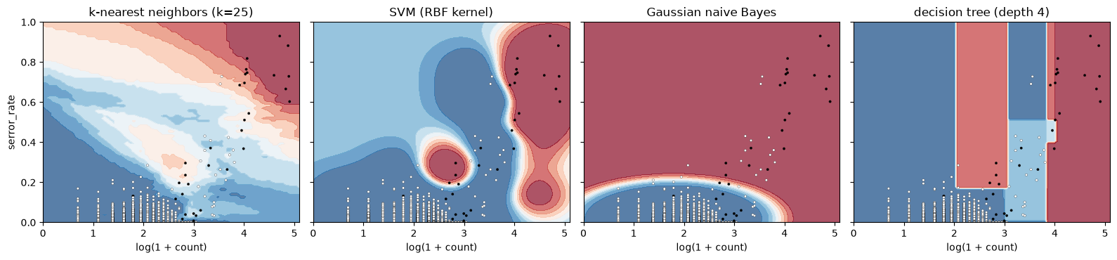
k-nearest neighbors and the tree follow the data locally, the tree with axis-parallel steps. The RBF support vector machine draws a smooth curved boundary. Gaussian naive Bayes models each feature with one normal distribution per class, so its boundary is a smooth quadratic curve that can misplace clusters that are not bell-shaped.
Try this
- Change
n_neighborsto 1 and to 200. Predict which way AP moves in each case before running. - Give the logistic regression
class_weight="balanced". Does its AP change much? Does its mean predicted probability (Lesson 2.3)? - Remove
serror_ratefrom the features and retrain the forest. Is the drop in AP close to the permutation importance printed above?
Results summary
These are the numbers quoted in the lesson text and the data used for the figures.
short = {"logistic regression": "lr", "k-nearest neighbors": "knn", "SVM (RBF kernel)": "svm",
         "Gaussian naive Bayes": "gnb", "decision tree": "tree", "random forest": "rf", "gradient boosting": "hgb"}
results = {
    "n_train": int(len(train)), "n_test": int(len(test)),
    "n_train_attacks": int(ytr.sum()), "n_test_attacks": int(yte.sum()),
    "n_test_c2beacon": int((family == "c2beacon").sum()),
    "recall20_ceiling": float(20 * n_days / yte.sum()),
    "best_model": best,
    "best_depth": str(best_depth),
    "noise_impurity": float(imp_impurity["noise"]),
    "noise_impurity_rank": noise_rank,
    "noise_permutation": float(imp_perm["noise"]),
    "n_features_noise": len(names_n),
    "top_perm_feature": perm.index[0],
    "top_perm_value": float(perm["mean"].iloc[0]),
    "second_perm_feature": perm.index[1],
    "second_perm_value": float(perm["mean"].iloc[1]),
    "depth1_test": float(depth_test[0]), "depth1_train": float(depth_train[0]),
    "depth_best_test": float(max(depth_test)),
    "depth_none_test": float(depth_test[-1]), "depth_none_train": float(depth_train[-1]),
    "l1_nonzero_smallest_C": int(np.sum(np.abs(np.array(path["l1"][0])) > 1e-8)),
    "path_C_min": float(Cs[0]), "path_C_max": float(Cs[-1]),
    "path_ap_l2_min_C": float(path_ap["l2"][0]), "path_ap_l2_max_C": float(path_ap["l2"][-1]),
    "path_ap_l2_C1": float(path_ap["l2"][list(Cs).index(1.0)]),
    "path_ap_train_l2_max_C": float(path_ap_train["l2"][-1]),
}
first_nz = next(i for i, c in enumerate(path["l1"]) if np.any(np.abs(np.array(c)) > 1e-8))
results["l1_first_C"] = float(Cs[first_nz])
results["l1_first_features"] = " and ".join(f"`{feature_names[numeric_idx[j]]}`" for j in np.flatnonzero(np.abs(np.array(path["l1"][first_nz])) > 1e-8))
results["l1_first_count"] = int(np.sum(np.abs(np.array(path["l1"][first_nz])) > 1e-8))
for name, s in short.items():
    results[f"ap_{s}"] = float(table.loc[name, "ap"])
    results[f"ap_{s}_sd"] = float(table.loc[name, "ap_sd"])
    results[f"recall20_{s}"] = float(table.loc[name, "recall20"])
    results[f"recall100_{s}"] = float(table.loc[name, "recall100"])
    results[f"recall100_{s}_sd"] = float(table.loc[name, "recall100_sd"])
    results[f"boot_lo_{s}"] = boot[name][0]
    results[f"boot_hi_{s}"] = boot[name][1]
    results[f"seconds_{s}"] = float(seconds[name])
    for f in fam_table.columns:
        results[f"fam_{f}_{s}"] = float(fam_table.loc[name, f])
for f in ["duration", "src_bytes", "dst_bytes", "packets", "count", "srv_count", "serror_rate", "failed_logins", "rerror_rate", "same_srv_rate", "dst_host_count"]:
    results[f"coef_{f}"] = float(coef[f])
for k_, v in results.items():
    print(f"{k_:<26} {v}")

export = {
    "models": [{"name": n, "ap": float(table.loc[n, "ap"]), "ap_sd": float(table.loc[n, "ap_sd"]),
                "recall100": float(table.loc[n, "recall100"]), "recall100_sd": float(table.loc[n, "recall100_sd"]),
                "boot": list(boot[n])} for n in NAMES],
    "family": {n: {f: float(fam_table.loc[n, f]) for f in fam_table.columns} for n in NAMES},
    "perm": {"features": list(perm.index), "mean": [float(v) for v in perm["mean"]], "sd": [float(v) for v in perm["sd"]]},
    "noise_compare": {"features": list(compare.index), "impurity": [float(v) for v in compare["impurity"]],
                      "permutation": [float(v) for v in compare["permutation"]]},
    "depth": {"depths": [str(d) for d in depths], "train": [float(v) for v in depth_train], "test": [float(v) for v in depth_test]},
    "path": {"C": [float(c) for c in Cs], "features": [feature_names[i] for i in numeric_idx],
             "l2": path["l2"], "l1": path["l1"], "ap_l2": [float(v) for v in path_ap["l2"]],
             "ap_l1": [float(v) for v in path_ap["l1"]], "ap_train_l2": [float(v) for v in path_ap_train["l2"]],
             "ap_train_l1": [float(v) for v in path_ap_train["l1"]]},
    "boundary": {"g0": [float(v) for v in g0], "g1": [float(v) for v in g1],
                 "prob": {n: np.round(P, 4).tolist() for n, P in grid_prob.items()},
                 "points": {"x": [float(v) for v in Z_tr[sub[:1500], 0]], "y": [float(v) for v in Z_tr[sub[:1500], 1]],
                            "label": [int(v) for v in ytr[sub[:1500]]]}},
}

# When the course build runs this notebook, it saves the numbers for the lesson pages.
if os.environ.get("COURSE_RESULTS"):
    import json
    with open(os.environ["COURSE_RESULTS"], "w") as f:
        json.dump({"results": results, "data": export}, f)
n_train 26275 n_test 10495 n_train_attacks 608 n_test_attacks 432 n_test_c2beacon 180 recall20_ceiling 0.18518518518518517 best_model random forest best_depth 6 noise_impurity 0.016019178727842212 noise_impurity_rank 14 noise_permutation 0.00027928900190448135 n_features_noise 25 top_perm_feature service top_perm_value 0.17582110182379068 second_perm_feature dst_host_count second_perm_value 0.09484528105436003 depth1_test 0.24732516257384443 depth1_train 0.30901941481993334 depth_best_test 0.520197244625252 depth_none_test 0.45809277074865734 depth_none_train 1.0 l1_nonzero_smallest_C 0 path_C_min 0.0001 path_C_max 100.0 path_ap_l2_min_C 0.4392455826250403 path_ap_l2_max_C 0.5216386941849573 path_ap_l2_C1 0.5183902438073352 path_ap_train_l2_max_C 0.7459444793304357 l1_first_C 0.001 l1_first_features `failed_logins` and `serror_rate` l1_first_count 2 ap_lr 0.5183902438073352 ap_lr_sd 0.0 recall20_lr 0.18518518518518517 recall100_lr 0.4861111111111111 recall100_lr_sd 0.0 boot_lo_lr 0.4675828612455199 boot_hi_lr 0.560716707879737 seconds_lr 0.6140279769897461 fam_scan_lr 0.9186046511627907 fam_bruteforce_lr 0.7831325301204819 fam_dos_lr 0.96 fam_exfil_lr 0.5151515151515151 fam_c2beacon_lr 0.005555555555555556 ap_knn 0.5710022761688985 ap_knn_sd 0.0 recall20_knn 0.18518518518518517 recall100_knn 0.5629225455614345 recall100_knn_sd 0.0 boot_lo_knn 0.5244933951390767 boot_hi_knn 0.6142662755906106 seconds_knn 0.46663737297058105 fam_scan_knn 1.0 fam_bruteforce_knn 0.9314400458978772 fam_dos_knn 1.0 fam_exfil_knn 0.9052429052429053 fam_c2beacon_knn 0.0 ap_svm 0.6129616548521396 ap_svm_sd 0.0 recall20_svm 0.18518518518518517 recall100_svm 0.5833333333333334 recall100_svm_sd 0.0 boot_lo_svm 0.5689195909330427 boot_hi_svm 0.6555518243496906 seconds_svm 1.2181379795074463 fam_scan_svm 0.9883720930232558 fam_bruteforce_svm 0.9518072289156626 fam_dos_svm 0.98 fam_exfil_svm 0.9393939393939394 fam_c2beacon_svm 0.044444444444444446 ap_gnb 0.3100912187571384 ap_gnb_sd 0.0 recall20_gnb 0.09259259259259259 recall100_gnb 0.46064814814814814 recall100_gnb_sd 0.0 boot_lo_gnb 0.2681582052002688 boot_hi_gnb 0.35103786859552316 seconds_gnb 0.026555299758911133 fam_scan_gnb 0.9069767441860465 fam_bruteforce_gnb 0.7349397590361446 fam_dos_gnb 1.0 fam_exfil_gnb 0.30303030303030304 fam_c2beacon_gnb 0.0 ap_tree 0.49967013299530383 ap_tree_sd 0.0034589565574013954 recall20_tree 0.17659571409362224 recall100_tree 0.5064814814814815 recall100_tree_sd 0.003803628871563652 boot_lo_tree 0.4510421688331389 boot_hi_tree 0.5448178599704351 seconds_tree 0.7565562725067139 fam_scan_tree 0.8651162790697674 fam_bruteforce_tree 0.8674698795180722 fam_dos_tree 0.9480000000000001 fam_exfil_tree 0.7575757575757576 fam_c2beacon_tree 0.0 ap_rf 0.7006590909097886 ap_rf_sd 0.010288452143163136 recall20_rf 0.18518518518518517 recall100_rf 0.6055555555555555 recall100_rf_sd 0.002639294965507279 boot_lo_rf 0.6528882139337111 boot_hi_rf 0.7316284741642691 seconds_rf 6.863900423049927 fam_scan_rf 0.9976744186046511 fam_bruteforce_rf 0.9638554216867469 fam_dos_rf 0.984 fam_exfil_rf 0.9636363636363636 fam_c2beacon_rf 0.08222222222222222 ap_hgb 0.6537603400125047 ap_hgb_sd 0.017281850042676537 recall20_hgb 0.18518518518518517 recall100_hgb 0.5685185185185185 recall100_hgb_sd 0.0020704333124997856 boot_lo_hgb 0.6120589371715293 boot_hi_hgb 0.6913794699649259 seconds_hgb 2.861454725265503 fam_scan_hgb 0.9883720930232558 fam_bruteforce_hgb 0.9566265060240964 fam_dos_hgb 1.0 fam_exfil_hgb 0.9454545454545455 fam_c2beacon_hgb 0.0 coef_duration 0.13050564995841346 coef_src_bytes 1.5237718514226244 coef_dst_bytes -0.0921750977783238 coef_packets -0.39492550793025283 coef_count 1.8545507266732724 coef_srv_count -0.43373562671272864 coef_serror_rate 0.41796821494138525 coef_failed_logins 0.4409506343383501 coef_rerror_rate -0.1003636652044222 coef_same_srv_rate -0.5344594087278742 coef_dst_host_count -1.0015422727605365