Unit 2 · Lesson 2.2
Splits, leakage and cross-validation
A score on held-out data is an estimate of how a detector will perform on data it has not seen. It is a good estimate only if the held-out data stands in the same relation to the training data as future traffic will stand to everything the detector learned from. In security that relation has three features that a random split ignores. The future contains attacks that did not exist in the past, records from the same host or campaign resemble one another, and some information that is easy to find in a stored dataset is not available at the moment a detector must decide. This lesson shows how to split data so that the test resembles deployment, how to use cross-validation without biasing the estimate, and how leakage, the use of information that would not be available in practice, inflates scores. Lab 2 measures each effect on the course dataset.
Training, validation and test sets
Supervised learning uses data for three different purposes. The training set is used to fit the parameters of a model, such as the coefficients of a logistic regression or the splits of a tree. The validation set is used to make choices that the training procedure does not make by itself, such as the regularization strength, the depth of a tree, which features to keep, which of several models to deploy, and the decision threshold. The test set is used once, at the end, to estimate the performance of the final choice.
The test estimate is unbiased only if nothing about the test set influenced any choice. Every time you look at a test score and change something in response, part of the test set becomes validation data, and the next test score is optimistic. Arp et al. (2022) call this test snooping and count it, together with temporal snooping and selective snooping, as data snooping, one of ten pitfalls they identify in published security research. They list biased parameter selection separately, giving as an example a detection threshold for a network intrusion detection system chosen from a ROC curve (Lesson 2.3) on the test set.
Cross-validation
When data is scarce, holding out a fixed validation set wastes training data and gives a noisy estimate. In \(K\)-fold cross-validation the training data is divided into \(K\) folds of roughly equal size. For each \(k = 1, \dots, K\) a model is trained on all folds except fold \(k\) and scored on fold \(k\), giving a score \(S_k\). The cross-validation estimate is the average,
Every record is used for scoring exactly once and for training \(K-1\) times. The spread of the \(S_k\) gives a rough sense of the uncertainty, although the folds share training data, so the \(S_k\) are not independent.
With rare attacks, a random fold may contain few or no attacks, and a metric such as average precision is then undefined or very noisy. Stratified cross-validation assigns records to folds so that each fold has about the same share of attacks as the whole. In the course dataset the first ten days contain 608 attack records after deduplication, so stratified five-fold cross-validation puts about a fifth of them in each fold. In a large experiment with C4.5 decision trees and naive Bayes on real datasets, Kohavi (1995) found ten-fold stratified cross-validation to be the best of the methods he compared for model selection on datasets similar to his.
Cross-validation inherits every assumption of the split it is built from. A stratified \(K\)-fold split assigns records to folds at random, so for security data it has the same weaknesses as a single random split, which the next three sections describe.
Grouped splits for records that belong together
Connections from one host are not independent draws. The same host runs the same software, talks to the same servers and, if it is compromised, produces many attack records of the same kind. In a random split some of a host's records land in training and others in testing, and the model can recognize the host's habits instead of learning what makes traffic malicious. Kapoor and Narayanan (2023) list non-independence between training and test samples as a form of leakage, with the example of different observations of the same patient appearing in both sets, and recommend splits that account for the dependence.
A grouped split assigns whole groups to one side. Scikit-learn provides GroupKFold, StratifiedGroupKFold and GroupShuffleSplit, which take an array of group labels such as src_host. The groups can also be campaigns, malware families, users, or the sites of an organization, depending on what the detector must generalize to.
Figure 2.4 contrasts three ways of splitting the course data.
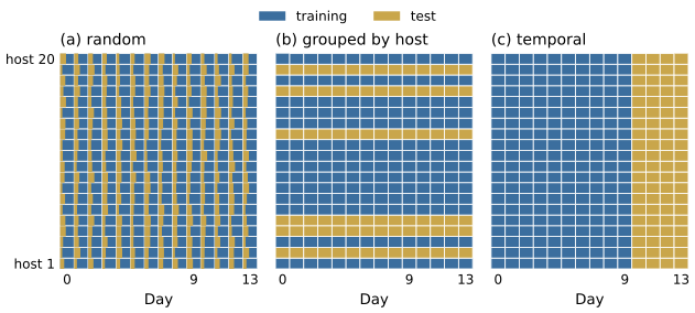
Figure 2.4. Three ways to split connection records, drawn as a grid of source hosts (rows, a sample of 20 of the 200 hosts) by days (columns). Each cell stands for the records of one host on one day, colored by the side it falls on. (a) A random split mixes training and test records within every cell. (b) A split grouped by host keeps every host entirely on one side. (c) A temporal split trains on days 0 to 9 and tests on days 10 to 13. Schematic; the proportions match the 70/30 and 10/4 splits used in Lab 2.
In Lab 2 the grouped split gives the gradient boosting detector an average precision (AP, Lesson 2.3) of 0.860, averaged over five seeds, with a standard deviation of 0.164. The individual seeds range from 0.533 to 0.952. The lowest value comes from the split in which host A010, which runs the IT team's authorized vulnerability scanner, falls into the test set (this happens for 1 of the five seeds). Its scans look like port scans, and a model that has never seen them labeled as normal puts 62 of them among its 100 highest-scored test records. With the records of A010 removed from that test set, the same model scores 0.949, in line with the other seeds, so this one host accounts for the low value. A random split hides this weakness because some of the scanner's records are always in training. The spread across seeds is a finding in itself. The score depends on which hosts happen to be held out, and a single grouped split would have given either a reassuring or an alarming number.
Temporal splits
Security data drifts. New malware families and attack tools appear, benign software is updated, and users change what they do. A detector deployed today is judged on tomorrow's traffic. Pendlebury et al. (2019) call evaluations that ignore this temporally biased. Their first constraint for a realistic evaluation of malware classifiers is temporal training consistency, which requires every training object to be strictly older than every test object, because violating it lets the classifier learn from the future. In their experiments on Android malware, a classifier with an F1 score of 0.91 under ten-fold cross-validation dropped to 0.58 when trained on older apps and tested on newer ones, with 10% malware in both sets.
For the course data the temporal split trains on days 0 to 9 and tests on days 10 to 13. It is harder than any random split for a concrete reason. The command-and-control family c2beacon appears only from day 10, so it is absent from training. The gradient boosting detector reaches an AP of 0.654 on the temporal split, against 0.936 on a random split of the same deduplicated records. Scored without the c2beacon records, the temporal model trained with seed 0, whose AP with them is 0.653, reaches 0.972. That comparison is only indicative, because removing the beacons also lowers the base rate of the test set from 4.1% to 2.4%, and AP depends on the base rate (Lesson 2.3).
Choosing hyperparameters on time-ordered data also needs time-ordered validation. Scikit-learn's TimeSeriesSplit, applied to rows sorted by time, produces folds in which each validation block follows its training block. A simpler scheme, used in Lab 2 to set a threshold, holds out the last days of the training period as a validation period.
Show the answer
First, random folds mix past and future, so the model is trained on samples from 2025 and tested on samples from 2023, and variants of a family seen in training appear in the test folds. Second, the share of malware in each fold equals the share in the collected dataset, which may be far higher than in the population the detector will see (the spatial bias of Pendlebury et al.). A temporally consistent evaluation trains on, say, 2023 and tests month by month on 2024 and 2025, with the malware share in each test month set to a realistic value, and chooses hyperparameters with validation data from the end of the training period.
Duplicates across the split
If a record appears twice and the copies fall on different sides of a random split, the test set contains a record the model has seen with its label. With \(D\) duplicated pairs and a split that puts each record in training with probability \(q\), the expected number of pairs split across the two sides is \(2q(1-q)D\). The course dataset has 1,103 rows that repeat an earlier row, and no record occurs more than twice, so \(D = 1{,}103\) and a random 70/30 split of the raw data is expected to leave \(2 \times 0.7 \times 0.3 \times 1{,}103 \approx 463\) test records with an identical copy in training.
The size of the resulting inflation depends on how many such records are attacks and on how well the model would have scored them anyway. Lab 2 isolates the effect by keeping one deduplicated test set and training twice, once on clean data and once with the twins of test records added to training. With 3% of records duplicated at random, an average of 5.2 of the 312 test attacks have a twin in training, and the AP of the gradient boosting detector changes by +0.0019 (standard deviation 0.0036 across five seeds), a change smaller than its own spread and so not measurable. The effect grows with the share of duplicates and when they are concentrated in the attack class. In the KDD Cup 1999 data, where most records were duplicates, Tavallaee et al. (2009) found that the test set was biased toward methods that detect the frequent records well. A temporal split happens to keep exact duplicates together, since they share a timestamp, but near-duplicates such as repacked malware samples cross time boundaries freely, which is why deduplication and grouping by family both matter.
Target leakage
Target leakage occurs when a feature carries information about the label that would not be available when the prediction is made. Kaufman et al. (2011) define leakage in general as the introduction of information about the target that should not be legitimately available to mine from, note that it is usually unintentional and introduced by the way data is collected, aggregated and prepared, and observe that at the very least it leads to overestimating the model's performance. They recommend tagging every observation with the time at which it became available and building models only from information that precedes the prediction, which they call a learn-predict separation. Kapoor and Narayanan (2023) list the use of features that are not legitimate as a separate category of leakage, and give a feature that is a proxy for the outcome as one instance.
The course dataset contains such a column on purpose. ticket_opened records whether an analyst opened a ticket after investigating the connection. It exists only after the decision the detector is supposed to make, and analysts open tickets for most attacks they see. Added as a feature, it raises the AP of the gradient boosting detector on the temporal split from 0.654 to 0.896, and that of the logistic regression from 0.519 to 0.861. In real data the leaked column is rarely labeled so clearly. Typical cases in security are a verdict from dynamic malware analysis or an antivirus scan run after the event, a field updated when an incident was closed, a feature computed over a window that extends past the event, and a blocklist downloaded after the labels were assigned.
Leakage through preprocessing (Lesson 2.1) belongs to the same family. Lab 2 shows that a scaler fitted on all days changes the AP of a logistic regression by only +0.0004, while a target encoding computed on all days lets a column of pure noise raise the test AP of the gradient boosting detector from 0.654 to 0.751. The difference lies in what the step learns. A mean and a standard deviation summarize the test set weakly; a per-category label average copies part of it.
Figure 2.5 and the table below collect the scores of Lab 2.
| Evaluation | Gradient boosting AP | Logistic regression AP |
|---|---|---|
| Random 70/30 split, raw data | 0.939 ± 0.007 | 0.679 ± 0.017 |
| Random 70/30 split, deduplicated | 0.936 ± 0.007 | 0.685 ± 0.007 |
| Split grouped by source host | 0.860 ± 0.164 | 0.680 ± 0.069 |
| Temporal split (days 0 to 9, then 10 to 13) | 0.654 ± 0.015 | 0.519 ± 0.000 |
Temporal split with ticket_opened |
0.896 ± 0.005 | 0.861 ± 0.000 |
Each entry is the mean ± standard deviation over five seeds. For the random and grouped splits the seed changes the split, and for the temporal split it changes only the model's internal randomness, so the logistic regression, which has none, shows zero spread there. The raw and deduplicated random splits give scores within about one standard deviation of each other, consistent with the controlled experiment above, which finds no measurable effect of the leaked twins. The temporal split is the setting that resembles deployment, and it gives the lowest score of all five rows for both detectors.
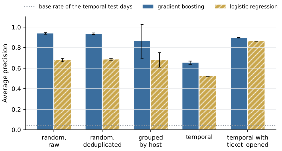
Figure 2.5. Average precision on held-out records of the same two detectors under the five evaluations of the table. Bars show the mean over five seeds and error bars one standard deviation. The dotted line is the base rate of the temporal test days, the AP of a detector that ranks records at random. Only the temporal split without ticket_opened mirrors deployment. Data from Lab 2.
Show the answer
Probably not. User reports accumulate after delivery, so at the moment the detector must decide (when the message arrives) the count is zero or very small. A temporal split by message date does not help, because the feature value stored in the dataset was computed later than the message date. The fix is to compute every feature as of the decision time (a learn-predict separation in the sense of Kaufman et al.), or to drop the feature.
Nested cross-validation against snooping in model selection
Choosing hyperparameters by cross-validation and reporting the best cross-validated score is a subtler form of snooping. The selection rewards the configuration whose folds happened to be favorable, so its score is biased upward. Cawley and Talbot (2010) show that this bias, which arises from overfitting the model selection criterion, can be of comparable size to the differences in performance between learning algorithms, and conclude that model selection must be treated as an integral part of fitting the model and repeated every time a model is fitted to a new sample of data, as in nested cross-validation.
Nested cross-validation has an outer loop that estimates performance and an inner loop that selects hyperparameters, as in Figure 2.6. For each outer fold, an inner cross-validation that uses only the outer training part chooses the hyperparameters, and the model refitted with them on the whole outer training part is scored on the outer test fold, which the selection never saw. The outer scores estimate the performance of the whole procedure, selection included. The cost multiplies. With five outer folds, five inner folds and ten candidate values of one hyperparameter, the procedure fits \(5 \times 5 \times 10 = 250\) models in the inner loops and 5 refits, 255 in all.
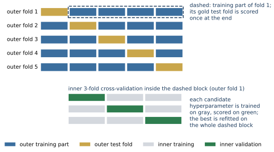
Figure 2.6. Nested cross-validation with five outer folds. Each outer fold (top rows) holds out one block as its test fold. Inside the training part of an outer fold (dashed, shown for fold 1), an inner cross-validation, here with three folds (bottom rows), compares candidate hyperparameters; the winner is refitted on the whole training part and scored once on the outer test fold. Schematic.
For time-ordered security data the same structure applies with temporal folds. The outer split trains on the past and tests on the next period, and the inner selection uses only data from within the outer training period. In practice a single temporal split with a validation period carved from the end of the training period, as in Lab 2, is often enough, provided the test period is looked at once.
What the lab shows
Lab 2
How leakage inflates a detector
Open in ColabRead with outputsNotebook on GitHubAbout 2 minutes to run on a laptop CPU
Lab 2 runs the split and leakage comparisons of this lesson on flows.csv, and Exercise 5 of this unit adds grouped and forward-chaining cross-validation to it. Change one thing at a time and predict the direction of the effect before running the cell.
Summary
A held-out score estimates deployed performance only if the held-out data relates to the training data as future traffic will. For security data that usually means a temporal split, so that new attack families and drift appear in the test as they do in practice, and a split grouped by host, campaign or family, so that the model cannot score well by recognizing the source. Stratification keeps rare attacks present in every fold. Exact duplicates should be removed before splitting; their effect on a score is small when they are few and spread evenly, and large when they dominate a dataset. Target leakage comes from features that exist only after the decision, and preprocessing leakage from learned steps fitted on all data, with supervised steps leaking far more than unsupervised ones. Selecting models or thresholds on the test set biases the estimate; nested cross-validation, or a separate validation period, keeps selection out of the final evaluation.
References
- Arp, D., Quiring, E., Pendlebury, F., Warnecke, A., Pierazzi, F., Wressnegger, C., Cavallaro, L., and Rieck, K. (2022). Dos and don'ts of machine learning in computer security. Proceedings of the 31st USENIX Security Symposium, 3971-3988. https://www.usenix.org/conference/usenixsecurity22/presentation/arp
- Cawley, G. C., and Talbot, N. L. C. (2010). On over-fitting in model selection and subsequent selection bias in performance evaluation. Journal of Machine Learning Research, 11, 2079-2107. https://www.jmlr.org/papers/v11/cawley10a.html
- Kapoor, S., and Narayanan, A. (2023). Leakage and the reproducibility crisis in machine-learning-based science. Patterns, 4(9), 100804. https://doi.org/10.1016/j.patter.2023.100804
- Kaufman, S., Rosset, S., and Perlich, C. (2011). Leakage in data mining: Formulation, detection, and avoidance. Proceedings of the 17th ACM SIGKDD International Conference on Knowledge Discovery and Data Mining, 556-563. https://doi.org/10.1145/2020408.2020496
- Kohavi, R. (1995). A study of cross-validation and bootstrap for accuracy estimation and model selection. Proceedings of the Fourteenth International Joint Conference on Artificial Intelligence (IJCAI), 1137-1143. https://www.ijcai.org/Proceedings/95-2/Papers/016.pdf
- Pendlebury, F., Pierazzi, F., Jordaney, R., Kinder, J., and Cavallaro, L. (2019). TESSERACT: Eliminating experimental bias in malware classification across space and time. Proceedings of the 28th USENIX Security Symposium, 729-746. https://www.usenix.org/conference/usenixsecurity19/presentation/pendlebury
- Tavallaee, M., Bagheri, E., Lu, W., and Ghorbani, A. A. (2009). A detailed analysis of the KDD CUP 99 data set. 2009 IEEE Symposium on Computational Intelligence for Security and Defense Applications, 1-6. https://doi.org/10.1109/CISDA.2009.5356528