# On Google Colab, install the scikit-learn version the course was built with.
# On your own computer, install requirements.txt instead; this cell then does nothing.
import subprocess, sys
if "google.colab" in sys.modules:
    subprocess.run([sys.executable, "-m", "pip", "install", "-q", "scikit-learn==1.9.0"], check=True)

Lab 2. How leakage inflates a detector

This lab measures how much the way you split and prepare data changes the score of the same detector. Every experiment uses the course dataset and the same two models, a histogram gradient boosting classifier and a logistic regression, and reports average precision (AP) on held-out records. Lessons 2.1 to 2.3 explain the ideas; here you see their size on real numbers. It runs in a few minutes on a laptop CPU.

You will:

1. find the duplicated records and measure what they do to a random split;
2. compare a random split, a split grouped by source host, and a split by time;
3. add a column that is only known after an analyst has looked at the alert;
4. fit preprocessing steps on all the data instead of on the training data only;
5. draw ROC and precision-recall curves for the time-ordered split;
6. choose a threshold from an alert budget of 20 alerts per day;
7. check whether the predicted probabilities are calibrated.

The data is synthetic (see Lesson 1.3). Most comparisons that depend on a random seed are repeated with five seeds and reported as the mean and the standard deviation. The cells that use a single gradient boosting model train it with seed 0.

import os
import warnings

import numpy as np
import pandas as pd
import matplotlib.pyplot as plt

from sklearn.calibration import CalibratedClassifierCV, calibration_curve
from sklearn.compose import ColumnTransformer
from sklearn.ensemble import HistGradientBoostingClassifier
from sklearn.frozen import FrozenEstimator
from sklearn.linear_model import LogisticRegression
from sklearn.metrics import average_precision_score, brier_score_loss, precision_recall_curve, roc_auc_score, roc_curve
from sklearn.model_selection import GroupShuffleSplit, StratifiedKFold, train_test_split
from sklearn.pipeline import make_pipeline
from sklearn.preprocessing import FunctionTransformer, OneHotEncoder, StandardScaler, TargetEncoder

warnings.filterwarnings("ignore")

LOCAL = "../../data/flows.csv"
URL = "https://raw.githubusercontent.com/aalbata/machine-learning-for-cybersecurity/main/data/flows.csv"
flows = pd.read_csv(LOCAL if os.path.exists(LOCAL) else URL)
SEEDS = [0, 1, 2, 3, 4]
print(flows.shape)

(37873, 21)

The features are those of Lab 1 plus the site. The byte and count columns are skewed, so they are log-transformed before scaling. The columns timestamp, day, src_host, attack_type, label and ticket_opened are not features.

skewed = ["duration", "src_bytes", "dst_bytes", "packets", "count", "srv_count"]
plain = ["failed_logins", "serror_rate", "rerror_rate", "same_srv_rate", "dst_host_count", "hour"]
categorical = ["protocol", "service", "site"]


def preprocessor(extra=()):
    return ColumnTransformer([
        ("log", make_pipeline(FunctionTransformer(np.log1p), StandardScaler()), skewed),
        ("num", StandardScaler(), plain + list(extra)),
        ("cat", OneHotEncoder(handle_unknown="ignore", sparse_output=False), categorical),
    ])


def make_model(kind, seed=0, extra=()):
    if kind == "hgb":
        return make_pipeline(preprocessor(extra), HistGradientBoostingClassifier(random_state=seed))
    return make_pipeline(preprocessor(extra), LogisticRegression(max_iter=3000))


def test_ap(kind, train, test, seed=0, extra=()):
    model = make_model(kind, seed, extra).fit(train, train["label"])
    return average_precision_score(test["label"], model.predict_proba(test)[:, 1])


def summary(values):
    return float(np.mean(values)), float(np.std(values))

1. Duplicated records

Collectors sometimes log the same connection twice. An exact duplicate has the same values in every column, including the timestamp.

dup_mask = flows.duplicated(keep=False)
n_dup_rows = int(flows.duplicated().sum())
print(f"rows that are an exact copy of an earlier row: {n_dup_rows:,} ({n_dup_rows / len(flows):.1%})")
dedup = flows.drop_duplicates().reset_index(drop=True)
print(f"after deduplication: {len(dedup):,} rows, base rate {dedup['label'].mean():.2%}")

rows that are an exact copy of an earlier row: 1,103 (2.9%)
after deduplication: 36,770 rows, base rate 2.83%

Deduplication needs no information from other rows' labels or statistics, so it can and should be done before splitting. What happens if we skip it? Below, a random stratified 70/30 split is made five times on the raw data and five times on the deduplicated data.

ap_split = {}
for name, df in [("random_raw", flows), ("random_dedup", dedup)]:
    for kind in ["hgb", "lr"]:
        vals = []
        for s in SEEDS:
            tr, te = train_test_split(df, test_size=0.3, stratify=df["label"], random_state=s)
            vals.append(test_ap(kind, tr, te, seed=s))
        ap_split[(name, kind)] = summary(vals)
        print(f"{name:<13} {kind}: AP {ap_split[(name, kind)][0]:.3f} +/- {ap_split[(name, kind)][1]:.3f}")

random_raw    hgb: AP 0.939 +/- 0.007

random_raw    lr: AP 0.679 +/- 0.017

random_dedup  hgb: AP 0.936 +/- 0.007

random_dedup  lr: AP 0.685 +/- 0.007

The two settings use different test sets, so their difference mixes the effect of copies of test records that sit in the training set with the effect of the different composition of the test sets. The next cell isolates the first effect. It keeps one deduplicated test set and trains twice, once on clean training data and once after adding the twins of test records that a raw random split would have put in training (each with probability 0.7, the training share).

twin_count = flows.groupby(list(flows.columns)).size().rename("copies").reset_index()
dedup_c = dedup.merge(twin_count, on=list(flows.columns), how="left")
twin_gain = {"hgb": [], "lr": []}
twin_attacks = []
for s in SEEDS:
    tr, te = train_test_split(dedup_c, test_size=0.3, stratify=dedup_c["label"], random_state=s)
    rng = np.random.default_rng(s)
    twins = te[te["copies"] == 2]
    twins = twins[rng.random(len(twins)) < 0.7]
    twin_attacks.append(int(twins["label"].sum()))
    leaky_train = pd.concat([tr, twins])
    for kind in ["hgb", "lr"]:
        twin_gain[kind].append(test_ap(kind, leaky_train, te, s) - test_ap(kind, tr, te, s))
n_test_attacks_random = int(te["label"].sum())
print(f"test attacks per split: {n_test_attacks_random}; of these with a twin in training: {np.mean(twin_attacks):.1f} on average")
for kind in ["hgb", "lr"]:
    m, sd = summary(twin_gain[kind])
    print(f"{kind}: change in AP from the leaked twins {m:+.4f} +/- {sd:.4f}")

test attacks per split: 312; of these with a twin in training: 5.2 on average
hgb: change in AP from the leaked twins +0.0019 +/- 0.0036
lr: change in AP from the leaked twins +0.0002 +/- 0.0003

With 3% duplicates spread at random, only a few of the roughly 300 test attacks have a twin in training, so even perfect memorization of those few can move AP only a little, and the measured change is smaller than its spread across seeds. It grows with the share of duplicates and when the duplicates are concentrated in the attack class, as they were in some public intrusion datasets.

2. Random, grouped and temporal splits

From here on the data is deduplicated. A grouped split puts all records of a source host on the same side, so the test hosts are hosts the model has never seen. A temporal split trains on days 0 to 9 and tests on days 10 to 13, which is how a detector is used.

scanner_top100 = []
for kind in ["hgb", "lr"]:
    vals, scanner_in_test = [], []
    for s in SEEDS:
        gss = GroupShuffleSplit(n_splits=1, test_size=0.3, random_state=s)
        a, b = next(gss.split(dedup, groups=dedup["src_host"]))
        tr, te = dedup.iloc[a], dedup.iloc[b]
        model = make_model(kind, s).fit(tr, tr["label"])
        sc = model.predict_proba(te)[:, 1]
        vals.append(average_precision_score(te["label"], sc))
        scanner_in_test.append("A010" in set(te["src_host"]))
        if kind == "hgb" and scanner_in_test[-1]:
            top = np.argsort(-sc)[:100]
            scanner_top100.append(int((te["src_host"].to_numpy()[top] == "A010").sum()))
            other = (te["src_host"] != "A010").to_numpy()
            ap_without_scanner = average_precision_score(te["label"][other], sc[other])
    ap_split[("grouped", kind)] = summary(vals)
    print(f"grouped {kind}: AP per seed {np.round(vals, 3)}, scanner host in test {scanner_in_test}")
    if kind == "hgb":
        grouped_hgb_vals = vals
        grouped_scanner = scanner_in_test
print("records of host A010 among the 100 highest-scored test records (seeds where it is in test):", scanner_top100)
print(f"gradient boosting AP of that split with the records of A010 removed from the test set: {ap_without_scanner:.3f}")

train = dedup[dedup["day"] <= 9]
test = dedup[dedup["day"] >= 10]
for kind in ["hgb", "lr"]:
    vals = [test_ap(kind, train, test, seed=s) for s in SEEDS]
    ap_split[("temporal", kind)] = summary(vals)
for key, (m, sd) in ap_split.items():
    print(f"{key[0]:<13} {key[1]}: AP {m:.3f} +/- {sd:.3f}")

grouped hgb: AP per seed [0.933 0.951 0.533 0.952 0.934], scanner host in test [False, False, True, False, False]

grouped lr: AP per seed [0.68  0.754 0.55  0.716 0.701], scanner host in test [False, False, True, False, False]
records of host A010 among the 100 highest-scored test records (seeds where it is in test): [62]
gradient boosting AP of that split with the records of A010 removed from the test set: 0.949

random_raw    hgb: AP 0.939 +/- 0.007
random_raw    lr: AP 0.679 +/- 0.017
random_dedup  hgb: AP 0.936 +/- 0.007
random_dedup  lr: AP 0.685 +/- 0.007
grouped       hgb: AP 0.860 +/- 0.164
grouped       lr: AP 0.680 +/- 0.069
temporal      hgb: AP 0.654 +/- 0.015
temporal      lr: AP 0.519 +/- 0.000

Host A010 runs the IT team's authorized vulnerability scanner. When a grouped split puts it in the test set, the model has never been told that scanning from this host is benign, and the cell shows how many of its records land among the 100 highest-scored test records. Removing the records of A010 from that test set gives a score in line with the other seeds, so this one host accounts for the low value. A random split hides this because some of the scanner's records are always in training. The spread across seeds of the grouped split is itself a finding, since the score depends on which hosts are held out.

The temporal split is harder for a different reason. The c2beacon family appears only from day 10. The next cell scores the temporal model without those records. Note that the base rate changes too, and AP depends on the base rate (Lesson 2.3), so the two AP values are not a clean comparison.

hgb_temporal = make_model("hgb", seed=0).fit(train, train["label"])
score = hgb_temporal.predict_proba(test)[:, 1]
known = (test["attack_type"] != "c2beacon").to_numpy()
ap_without_c2 = average_precision_score(test["label"][known], score[known])
print(f"test base rate {test['label'].mean():.2%}; without c2beacon {test['label'][known].mean():.2%}")
print(f"AP with c2beacon {average_precision_score(test['label'], score):.3f}; without {ap_without_c2:.3f}")

test base rate 4.12%; without c2beacon 2.44%
AP with c2beacon 0.653; without 0.972

3. Target leakage

ticket_opened records whether an analyst opened a ticket. It is filled in after investigation, so a deployed detector cannot see it. Adding it as a feature shows how much a leaked column can inflate a score.

leak = {}
for kind in ["hgb", "lr"]:
    vals = [test_ap(kind, train, test, seed=s, extra=["ticket_opened"]) for s in SEEDS]
    leak[kind] = summary(vals)
    print(f"temporal {kind} with ticket_opened: AP {leak[kind][0]:.3f} +/- {leak[kind][1]:.3f}"
          f" (without: {ap_split[('temporal', kind)][0]:.3f})")

temporal hgb with ticket_opened: AP 0.896 +/- 0.005 (without: 0.654)

temporal lr with ticket_opened: AP 0.861 +/- 0.000 (without: 0.519)

4. Preprocessing fitted on all the data

The first experiment concerns an unsupervised step. The scalers and the one-hot encoder are fitted on all 14 days, test days included, and the logistic regression is then trained on days 0 to 9 as before.

prep_all = preprocessor().fit(dedup)
lr_all = LogisticRegression(max_iter=3000).fit(prep_all.transform(train), train["label"])
ap_scaler_all = average_precision_score(test["label"], lr_all.predict_proba(prep_all.transform(test))[:, 1])
ap_scaler_pipe = ap_split[("temporal", "lr")][0]
print(f"scaler fitted inside the pipeline (training days only): AP {ap_scaler_pipe:.4f}")
print(f"scaler fitted on all days:                          AP {ap_scaler_all:.4f}")
print(f"difference: {ap_scaler_all - ap_scaler_pipe:+.4f}")

scaler fitted inside the pipeline (training days only): AP 0.5194
scaler fitted on all days:                          AP 0.5198
difference: +0.0004

The difference is tiny. A scaler learns only a mean and a standard deviation per column, which the 10,495 rows of the test days barely move, and a shift or rescaling of a feature changes a logistic regression only through its penalty. The rule still holds, because other steps learn far more from the data. A supervised step, one that uses the labels, can leak a great deal.

To show this, we add a synthetic identifier column conn_id with 2,000 random values that carry no information about the label (think of a connection or flow identifier) and target-encode it in three ways:

• the naive encoding uses the smoothed mean label of each identifier, computed on the training rows and applied to those same rows (TargetEncoder.fit followed by transform);
• the cross-fitted encoding uses scikit-learn's TargetEncoder, whose fit_transform encodes each training row with statistics from the other folds;
• the naive encoding on all days uses the smoothed mean label of each identifier computed on all 14 days, test days included, which is what happens when the encoding is done before the split.

rng = np.random.default_rng(0)
conn_id = rng.integers(0, 2000, len(dedup)).astype(str)
train_id = conn_id[(dedup["day"] <= 9).to_numpy()].reshape(-1, 1)
test_id = conn_id[(dedup["day"] >= 10).to_numpy()].reshape(-1, 1)
base_prep = preprocessor().fit(train)
Xtr, Xte = base_prep.transform(train), base_prep.transform(test)
ytr, yte = train["label"].to_numpy(), test["label"].to_numpy()

encodings = {}
naive = TargetEncoder(target_type="binary").fit(train_id, ytr)
encodings["naive"] = (naive.transform(train_id), naive.transform(test_id))
cross = TargetEncoder(target_type="binary", cv=StratifiedKFold(5, shuffle=True, random_state=0))
encodings["cross-fitted"] = (cross.fit_transform(train_id, ytr), cross.transform(test_id))
all_id = np.vstack([train_id, test_id])
all_y = np.concatenate([ytr, yte])
everything = TargetEncoder(target_type="binary").fit(all_id, all_y)
encodings["naive on all days"] = (everything.transform(train_id), everything.transform(test_id))

te_ap = {"none": []}
for s in SEEDS:
    m = HistGradientBoostingClassifier(random_state=s).fit(Xtr, ytr)
    te_ap["none"].append(average_precision_score(yte, m.predict_proba(Xte)[:, 1]))
for name, (a, b) in encodings.items():
    te_ap[name] = []
    for s in SEEDS:
        m = HistGradientBoostingClassifier(random_state=s).fit(np.hstack([Xtr, a]), ytr)
        te_ap[name].append(average_precision_score(yte, m.predict_proba(np.hstack([Xte, b]))[:, 1]))
for name, vals in te_ap.items():
    print(f"conn_id {name:<20} AP {np.mean(vals):.3f} +/- {np.std(vals):.3f}")

conn_id none                 AP 0.654 +/- 0.015
conn_id naive                AP 0.256 +/- 0.006
conn_id cross-fitted         AP 0.649 +/- 0.012
conn_id naive on all days    AP 0.751 +/- 0.013

The naive encoding gives every training row a value computed partly from its own label. With about 13 rows per identifier, that value separates attacks from normal records in training, the model relies on it, and on the test days, where the column carries no information, the detector falls apart. Cross-fitting removes the effect, because the model learns that the column is useless and ignores it. When the naive encoding is computed before the split, the test rows are encoded with their own labels as well, and the same useless column now raises the test score above the leakage-free one. Nothing about the detector improved; the score measures the leak.

5. ROC and precision-recall curves for the temporal split

This section and the first cell of Section 6 use the gradient boosting model trained on days 0 to 9 with seed 0 (hgb_temporal above), and this section also uses a logistic regression trained the same way. The second cell of Section 6 and Section 7 train new models on days 0 to 7.

lr_temporal = make_model("lr").fit(train, train["label"])
scores = {"hgb": score, "lr": lr_temporal.predict_proba(test)[:, 1]}
prevalence_test = float(yte.mean())
curves = {}
fig, axes = plt.subplots(1, 2, figsize=(10, 4))
for kind, sc in scores.items():
    fpr, tpr, _ = roc_curve(yte, sc)
    prec, rec, _ = precision_recall_curve(yte, sc)
    curves[kind] = dict(fpr=fpr, tpr=tpr, precision=prec, recall=rec,
                        auc=roc_auc_score(yte, sc), ap=average_precision_score(yte, sc))
    axes[0].plot(fpr, tpr, label=f"{kind}, AUC {curves[kind]['auc']:.3f}")
    axes[1].step(rec, prec, where="post", label=f"{kind}, AP {curves[kind]['ap']:.3f}")
axes[0].plot([0, 1], [0, 1], ":", color="gray", label="random ranking")
axes[1].axhline(prevalence_test, ls=":", color="gray", label=f"base rate {prevalence_test:.3f}")
axes[0].set_xlabel("False positive rate")
axes[0].set_ylabel("True positive rate (recall)")
axes[1].set_xlabel("Recall")
axes[1].set_ylabel("Precision")
axes[0].legend()
axes[1].legend()
plt.tight_layout()
plt.show()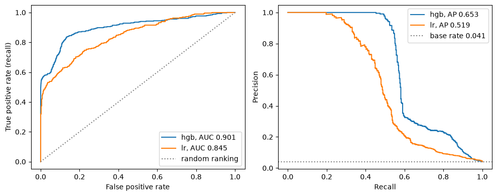

The ROC curve does not depend on the base rate, but the precision-recall curve does. To see how AP would change if attacks were rarer, we give every normal test record a weight, so that the weighted share of attacks equals a chosen base rate. The true and false positive rates at each threshold stay the same; only precision changes.

ap_at, pr_at = {}, {}
for target in [prevalence_test, 0.01, 0.001]:
    n_pos, n_neg = yte.sum(), (1 - yte).sum()
    w_neg = n_pos * (1 - target) / (target * n_neg)
    weights = np.where(yte == 1, 1.0, w_neg)
    ap_at[target] = {kind: average_precision_score(yte, sc, sample_weight=weights) for kind, sc in scores.items()}
    prec_w, rec_w, _ = precision_recall_curve(yte, scores["hgb"], sample_weight=weights)
    pr_at[target] = (rec_w, prec_w)
    print(f"base rate {target:.3%}: AP gradient boosting {ap_at[target]['hgb']:.3f}, logistic regression {ap_at[target]['lr']:.3f}")

base rate 4.116%: AP gradient boosting 0.653, logistic regression 0.519
base rate 1.000%: AP gradient boosting 0.571, logistic regression 0.398
base rate 0.100%: AP gradient boosting 0.504, logistic regression 0.266

6. A threshold from an alert budget

Suppose analysts can investigate 20 alerts per day. Over the four test days that is 80 alerts. The first cell below finds the threshold that produces exactly 80 alerts on the test days. That threshold is chosen by looking at the test data, so it shows the best this ranking can do within the budget; it is not something you could set in advance.

budget_per_day = 20
n_days_test = test["day"].nunique()
k = budget_per_day * n_days_test
order = np.argsort(-score)
threshold_oracle = float(score[order[k - 1]])
alert = score >= threshold_oracle
recall_budget = float(alert[yte == 1].mean())
precision_budget = float(yte[alert].mean())
print(f"threshold {threshold_oracle:.4f}: {alert.sum()} alerts, recall {recall_budget:.3f}, precision {precision_budget:.3f}")
recall_budget_family = {}
for fam in ["bruteforce", "c2beacon", "dos", "exfil", "scan"]:
    mask = (test["attack_type"] == fam).to_numpy()
    recall_budget_family[fam] = float(alert[mask].mean())
    print(f"  {fam:<11} recall {recall_budget_family[fam]:.2f}")

threshold 0.9997: 80 alerts, recall 0.185, precision 1.000
  bruteforce  recall 0.22
  c2beacon    recall 0.00
  dos         recall 0.66
  exfil       recall 0.00
  scan        recall 0.34

In practice the threshold must be set before the test days. The next cell trains on days 0 to 7, sets the threshold so that days 8 and 9 together produce 40 alerts, 20 per day on average, and then applies that fixed threshold to days 10 to 13.

early = dedup[dedup["day"] <= 7]
valid = dedup[dedup["day"].isin([8, 9])]
hgb_early = make_model("hgb", seed=0).fit(early, early["label"])
valid_score = np.sort(hgb_early.predict_proba(valid)[:, 1])[::-1]
threshold_valid = float(valid_score[budget_per_day * 2 - 1])
test_score_early = hgb_early.predict_proba(test)[:, 1]
alert_v = test_score_early >= threshold_valid
alerts_per_day_v = pd.Series(alert_v).groupby(test["day"].to_numpy()).sum()
recall_valid_threshold = float(alert_v[yte == 1].mean())
precision_valid_threshold = float(yte[alert_v].mean())
alerts_valid_dos = int((alert_v & (test["attack_type"] == "dos").to_numpy()).sum())
print(f"threshold set on days 8 and 9: {threshold_valid:.4f}")
print("alerts per test day:", alerts_per_day_v.to_dict())
print(f"recall on the test days {recall_valid_threshold:.3f}, precision {precision_valid_threshold:.3f}")
print("alerts on the test days by family:", test["attack_type"][alert_v].value_counts().to_dict())

threshold set on days 8 and 9: 0.9907
alerts per test day: {10: 22, 11: 65, 12: 27, 13: 23}
recall on the test days 0.317, precision 1.000
alerts on the test days by family: {'scan': 53, 'dos': 43, 'bruteforce': 39, 'exfil': 2}

The fixed threshold does not keep to the budget on the test days. The precision printed above is 1, so every alert is an attack, and the overrun is caused by attacks that score above the threshold, most of all the denial-of-service burst on day 11, and not by benign traffic. A threshold fixes a score, not a number of alerts, and the number of records above it changes from day to day with the volume of attacks and of attack-like benign traffic. Monitoring the daily alert count is part of operating a detector.

7. Calibration

A model is calibrated if, among records given probability \(p\), a share of about \(p\) are attacks. We train two logistic regressions on days 0 to 7, one plain and one with class_weight="balanced", and recalibrate the balanced one on days 8 and 9 with isotonic regression and with Platt (sigmoid) scaling, which gives four models. Calibration is then measured on days 10 to 13.

lr_plain = make_model("lr").fit(early, early["label"])
lr_bal = make_pipeline(preprocessor(), LogisticRegression(max_iter=3000, class_weight="balanced")).fit(early, early["label"])
iso = CalibratedClassifierCV(FrozenEstimator(lr_bal), method="isotonic").fit(valid, valid["label"])
platt = CalibratedClassifierCV(FrozenEstimator(lr_bal), method="sigmoid").fit(valid, valid["label"])
calib = {}
fig, ax = plt.subplots(figsize=(5, 4.5))
for name, m in [("plain", lr_plain), ("balanced", lr_bal), ("balanced + isotonic", iso), ("balanced + Platt", platt)]:
    p = m.predict_proba(test)[:, 1]
    frac_pos, mean_pred = calibration_curve(yte, p, n_bins=10, strategy="uniform")
    counts = np.histogram(p, bins=np.linspace(0, 1, 11))[0]
    calib[name] = dict(frac_pos=frac_pos, mean_pred=mean_pred, counts=counts[counts > 0],
                       brier=brier_score_loss(yte, p), mean_p=float(p.mean()),
                       ap=average_precision_score(yte, p))
    ax.plot(mean_pred, frac_pos, "o-", label=name)
    print(f"{name:<20} mean predicted {p.mean():.3f}  Brier {calib[name]['brier']:.4f}  AP {calib[name]['ap']:.3f}")
print(f"actual share of attacks on the test days: {prevalence_test:.3f}")
ax.plot([0, 1], [0, 1], ":", color="gray")
ax.set_xlabel("Mean predicted probability in bin")
ax.set_ylabel("Share of attacks in bin")
ax.legend()
plt.show()

plain                mean predicted 0.022  Brier 0.0261  AP 0.523
balanced             mean predicted 0.081  Brier 0.0462  AP 0.490
balanced + isotonic  mean predicted 0.017  Brier 0.0303  AP 0.451
balanced + Platt     mean predicted 0.016  Brier 0.0300  AP 0.490
actual share of attacks on the test days: 0.041

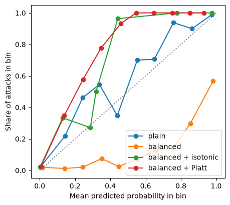
Balanced class weights make the model act as if attacks were as common as normal records, so its probabilities are too high. Compare its mean predicted probability with the actual share of attacks printed on the last line. Recalibration on days 8 and 9 brings the mean prediction down to about the base rate of those days, which is lower than that of the test days. Platt scaling is a monotone map, so it leaves the ranking and the AP unchanged. Isotonic regression is a step function, which merges many scores into ties, and here that costs AP. None of the curves is perfect on the test days. The c2beacon family, absent from both the training and the calibration days, accounts for part of this, since almost all of its records fall in the lowest bin and raise the share of attacks there. The higher bins, which contain almost no beacons, also deviate from the diagonal, so a calibration fitted on days 8 and 9 does not carry over exactly to the test days.

Try this

• Change test_size in the grouped split to 0.5. Predict whether the spread across seeds grows or shrinks, then check.
• Replace 2,000 by 200 identifiers in conn_id. With about 130 rows per identifier, how much damage does the naive encoding still do?
• Set the budget to 5 alerts per day. Which families disappear from the alerts first?
• Use strategy="quantile" in calibration_curve. Why do the bins look different for a rare class?

Results summary

These are the numbers quoted in the lesson text, and the curve data used for the figures.

def thin(x, y, n=300):
    """Keep at most n points of a curve, always including both ends."""
    idx = np.unique(np.linspace(0, len(x) - 1, min(n, len(x))).round().astype(int))
    return [float(v) for v in np.asarray(x)[idx]], [float(v) for v in np.asarray(y)[idx]]


results = {
    "n_records": int(len(flows)),
    "n_duplicates": n_dup_rows,
    "dup_share": n_dup_rows / len(flows),
    "n_dedup": int(len(dedup)),
    "n_train_temporal": int(len(train)),
    "n_test_temporal": int(len(test)),
    "n_test_attacks_temporal": int(yte.sum()),
    "prevalence_test": prevalence_test,
    "twin_attacks_mean": float(np.mean(twin_attacks)),
    "n_test_attacks_random": n_test_attacks_random,
    "twin_gain_hgb": summary(twin_gain["hgb"])[0],
    "twin_gain_hgb_sd": summary(twin_gain["hgb"])[1],
    "twin_gain_lr": summary(twin_gain["lr"])[0],
    "twin_gain_lr_sd": summary(twin_gain["lr"])[1],
    "grouped_hgb_min": float(np.min(grouped_hgb_vals)),
    "grouped_hgb_max": float(np.max(grouped_hgb_vals)),
    "grouped_scanner_seeds": int(np.sum(grouped_scanner)),
    "grouped_scanner_top100": int(scanner_top100[0]) if scanner_top100 else 0,
    "grouped_hgb_without_scanner": float(ap_without_scanner) if scanner_top100 else float("nan"),
    "ap_without_c2": float(ap_without_c2),
    "prevalence_without_c2": float(yte[known].mean()),
    "ap_scaler_pipe": float(ap_scaler_pipe),
    "ap_scaler_all": float(ap_scaler_all),
    "ap_scaler_diff": float(ap_scaler_all - ap_scaler_pipe),
    "auc_hgb": float(curves["hgb"]["auc"]),
    "ap_hgb": float(curves["hgb"]["ap"]),
    "auc_lr": float(curves["lr"]["auc"]),
    "ap_hgb_at_1pct": float(ap_at[0.01]["hgb"]),
    "ap_hgb_at_0_1pct": float(ap_at[0.001]["hgb"]),
    "ap_lr_at_1pct": float(ap_at[0.01]["lr"]),
    "ap_lr_at_0_1pct": float(ap_at[0.001]["lr"]),
    "ap_lr": float(curves["lr"]["ap"]),
    "budget_per_day": budget_per_day,
    "budget_alerts": int(k),
    "threshold_oracle": threshold_oracle,
    "recall_budget": recall_budget,
    "precision_budget": precision_budget,
    "threshold_valid": threshold_valid,
    "recall_valid_threshold": recall_valid_threshold,
    "precision_valid_threshold": precision_valid_threshold,
    "alerts_valid_dos": alerts_valid_dos,
    "alerts_per_day_valid_min": int(alerts_per_day_v.min()),
    "alerts_per_day_valid_max": int(alerts_per_day_v.max()),
    "alerts_valid_total": int(alert_v.sum()),
}
for key, (m, sd) in ap_split.items():
    results[f"ap_{key[0]}_{key[1]}"] = m
    results[f"ap_{key[0]}_{key[1]}_sd"] = sd
for kind in ["hgb", "lr"]:
    results[f"ap_leak_{kind}"] = leak[kind][0]
    results[f"ap_leak_{kind}_sd"] = leak[kind][1]
for name, short in [("none", "none"), ("naive", "naive"), ("cross-fitted", "cross"), ("naive on all days", "all")]:
    results[f"te_ap_{short}"] = float(np.mean(te_ap[name]))
    results[f"te_ap_{short}_sd"] = float(np.std(te_ap[name]))
for fam, v in recall_budget_family.items():
    results[f"recall_budget_{fam}"] = v
for name, short in [("plain", "plain"), ("balanced", "bal"), ("balanced + isotonic", "iso"), ("balanced + Platt", "platt")]:
    results[f"brier_{short}"] = float(calib[name]["brier"])
    results[f"meanp_{short}"] = float(calib[name]["mean_p"])
    results[f"calib_ap_{short}"] = float(calib[name]["ap"])
for k_, v in results.items():
    print(f"{k_:<28} {v}")

export = {"ap_table": {f"{a}|{b}": list(v) for (a, b), v in ap_split.items()},
          "leak": {kind: list(v) for kind, v in leak.items()},
          "te_ap": {name: [float(x) for x in vals] for name, vals in te_ap.items()},
          "budget_point": {"fpr": float(alert[yte == 0].mean()), "tpr": recall_budget,
                           "precision": precision_budget}}
for kind in ["hgb", "lr"]:
    fx, fy = thin(curves[kind]["fpr"], curves[kind]["tpr"])
    rx, ry = thin(curves[kind]["recall"], curves[kind]["precision"])
    export[f"roc_{kind}"] = {"fpr": fx, "tpr": fy}
    export[f"pr_{kind}"] = {"recall": rx, "precision": ry}
export["pr_hgb_at"] = [{"base_rate": float(t), "recall": thin(r_, p_)[0], "precision": thin(r_, p_)[1]}
                       for t, (r_, p_) in pr_at.items()]
export["calibration"] = {name: {"mean_pred": [float(v) for v in c["mean_pred"]],
                                "frac_pos": [float(v) for v in c["frac_pos"]],
                                "counts": [int(v) for v in c["counts"]]} for name, c in calib.items()}

# When the course build runs this notebook, it saves the numbers for the lesson pages.
if os.environ.get("COURSE_RESULTS"):
    import json
    with open(os.environ["COURSE_RESULTS"], "w") as f:
        json.dump({"results": results, "data": export}, f)

n_records                    37873
n_duplicates                 1103
dup_share                    0.029123650093734323
n_dedup                      36770
n_train_temporal             26275
n_test_temporal              10495
n_test_attacks_temporal      432
prevalence_test              0.041162458313482614
twin_attacks_mean            5.2
n_test_attacks_random        312
twin_gain_hgb                0.0018644912744365083
twin_gain_hgb_sd             0.0036135029113511016
twin_gain_lr                 0.0002364324119819683
twin_gain_lr_sd              0.00029238335641864157
grouped_hgb_min              0.5327482433583006
grouped_hgb_max              0.9516970768512258
grouped_scanner_seeds        1
grouped_scanner_top100       62
grouped_hgb_without_scanner  0.949311907624285
ap_without_c2                0.9718221891720186
prevalence_without_c2        0.02443044110518662
ap_scaler_pipe               0.5194242663622874
ap_scaler_all                0.5197755286916866
ap_scaler_diff               0.00035126232939919344
auc_hgb                      0.9009681138457348
ap_hgb                       0.6526111869723435
auc_lr                       0.8452062193366973
ap_hgb_at_1pct               0.5710250860922897
ap_hgb_at_0_1pct             0.5039839557647248
ap_lr_at_1pct                0.3984209557056428
ap_lr_at_0_1pct              0.26605193309229813
ap_lr                        0.5194242663622874
budget_per_day               20
budget_alerts                80
threshold_oracle             0.9997407955498582
recall_budget                0.18518518518518517
precision_budget             1.0
threshold_valid              0.990743428975357
recall_valid_threshold       0.31712962962962965
precision_valid_threshold    1.0
alerts_valid_dos             43
alerts_per_day_valid_min     22
alerts_per_day_valid_max     65
alerts_valid_total           137
ap_random_raw_hgb            0.9392523302020119
ap_random_raw_hgb_sd         0.007474491239455424
ap_random_raw_lr             0.6788823749234429
ap_random_raw_lr_sd          0.016558372380575455
ap_random_dedup_hgb          0.9362455569153155
ap_random_dedup_hgb_sd       0.007354085659564408
ap_random_dedup_lr           0.6847801701735616
ap_random_dedup_lr_sd        0.007214065142470773
ap_grouped_hgb               0.8603960265294937
ap_grouped_hgb_sd            0.16402606489366414
ap_grouped_lr                0.6801631709297074
ap_grouped_lr_sd             0.06948171755999609
ap_temporal_hgb              0.6537603400125047
ap_temporal_hgb_sd           0.015457356588952944
ap_temporal_lr               0.5194242663622874
ap_temporal_lr_sd            0.0
ap_leak_hgb                  0.8960720518838432
ap_leak_hgb_sd               0.005198056530098905
ap_leak_lr                   0.8610426012006052
ap_leak_lr_sd                0.0
te_ap_none                   0.6537603400125047
te_ap_none_sd                0.015457356588952944
te_ap_naive                  0.2564507735725584
te_ap_naive_sd               0.006244129047341553
te_ap_cross                  0.6494634063095571
te_ap_cross_sd               0.012192084972862428
te_ap_all                    0.7507705652074744
te_ap_all_sd                 0.012678297466071615
recall_budget_bruteforce     0.21686746987951808
recall_budget_c2beacon       0.0
recall_budget_dos            0.66
recall_budget_exfil          0.0
recall_budget_scan           0.3372093023255814
brier_plain                  0.02608841597613807
meanp_plain                  0.021510652231572294
calib_ap_plain               0.5234374662443027
brier_bal                    0.04621653134451637
meanp_bal                    0.08068199188723552
calib_ap_bal                 0.4901911233200179
brier_iso                    0.030296504987131757
meanp_iso                    0.01677170758985732
calib_ap_iso                 0.45066553726037956
brier_platt                  0.029956768373200042
meanp_platt                  0.01631406760885912
calib_ap_platt               0.4901911233200179