Unit 2 · Lesson 2.3
ROC and precision-recall curves, and choosing a threshold
Most classifiers do not output a decision. They output a score, such as a predicted probability of attack or a distance from a decision boundary, and an alert is raised when the score exceeds a threshold. Every threshold gives a different confusion matrix, so a single precision or recall describes one operating point of a detector, not the detector. This lesson describes all operating points at once with two curves, the receiver operating characteristic (ROC) curve and the precision-recall curve, explains how each depends on the base rate, and then shows how to choose the operating point at which a security team runs the detector, either from an alert budget or from the costs of errors. Choosing from costs requires calibrated probabilities, so the lesson ends with calibration.
The ROC curve and its area
Sort the test records by decreasing score and lower the threshold step by step. At each threshold, compute the true positive rate (recall) and the false positive rate of Lesson 1.2. The ROC curve plots the true positive rate against the false positive rate for every threshold, from \((0, 0)\), where nothing is flagged, to \((1, 1)\), where everything is. A detector that ranks records at random follows the diagonal, and a perfect ranking goes straight up to \((0, 1)\) and then across.
The area under the ROC curve (AUC) summarizes the whole curve in one number. It has a direct interpretation. Fawcett (2006) notes that the AUC equals the probability that the classifier scores a randomly chosen positive record above a randomly chosen negative one. With \(N_+\) attacks with scores \(s^+_i\) and \(N_-\) normal records with scores \(s^-_j\), the empirical AUC is
where \(\mathbb{1}[\cdot]\) is 1 when the condition holds and 0 otherwise, so ties count one half. An AUC of 0.5 is a random ranking and 1 a perfect one.
A worked example
Eight test records have the scores and labels in the table below, three attacks (A) and five normal records (N), so the base rate is \(3/8 = 0.375\).
| Rank | Score | Label | Recall | False positive rate | Precision |
|---|---|---|---|---|---|
| 1 | 0.92 | A | 1/3 | 0 | 1 |
| 2 | 0.81 | N | 1/3 | 1/5 | 1/2 |
| 3 | 0.74 | A | 2/3 | 1/5 | 2/3 |
| 4 | 0.60 | N | 2/3 | 2/5 | 2/4 |
| 5 | 0.55 | N | 2/3 | 3/5 | 2/5 |
| 6 | 0.43 | A | 1 | 3/5 | 3/6 |
| 7 | 0.30 | N | 1 | 4/5 | 3/7 |
| 8 | 0.12 | N | 1 | 1 | 3/8 |
Each row of the table is one threshold, set at the score in that row so that it flags the records of that rank and above. The last three columns give the recall, false positive rate and precision at that threshold. The ROC curve passes through \((0, 0)\), \((0, 1/3)\), \((0.2, 1/3)\), \((0.2, 2/3)\), \((0.4, 2/3)\), \((0.6, 2/3)\), \((0.6, 1)\), \((0.8, 1)\) and \((1, 1)\). To compute the AUC from \eqref{eq:auc}, count for each attack the normal records ranked below it. The attack at rank 1 is above all five, the one at rank 3 is above four (ranks 4, 5, 7 and 8), and the one at rank 6 is above two. That gives \(5 + 4 + 2 = 11\) correctly ordered pairs out of \(3 \times 5 = 15\), so \(\mathrm{AUC} = 11/15 \approx 0.733\), which is also the area under the staircase in Figure 2.7(a).
The precision-recall curve and average precision
The precision-recall curve plots precision against recall for every threshold. Its natural summary is average precision (AP). Scikit-learn computes it as
where \(P_n\) and \(R_n\) are the precision and recall at the \(n\)-th threshold in decreasing order of score and \(R_0 = 0\). Recall changes only when an attack is passed, by \(1/N_+\) each time, so when all scores are distinct, AP is the mean of the precision values at the ranks of the attacks. In the example these are 1 at rank 1, \(2/3\) at rank 3 and \(3/6\) at rank 6, so
Equation \eqref{eq:ap} is a step-wise sum, and it differs from the area obtained by joining the points of the precision-recall curve with straight lines, starting from the point \((0, 1)\), and applying the trapezoidal rule, which for the example gives 0.678. The difference is not a matter of numerical accuracy. Davis and Goadrich (2006) show that linear interpolation between points in precision-recall space is incorrect, because the precision achievable between two operating points does not in general lie on the straight line joining them. This course therefore reports AP as defined in \eqref{eq:ap} and does not call it an area under the precision-recall curve. Figure 2.7 draws both curves for the example.
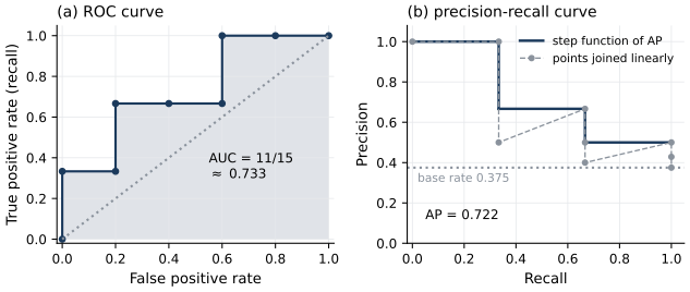
Figure 2.7. The worked example of eight scored records (three attacks). (a) ROC curve; the shaded area is the AUC of \(11/15 \approx 0.733\) and the dotted diagonal is a random ranking. (b) Precision-recall curve drawn as the step function used by average precision (solid), whose weighted sum gives AP = 0.722, with the points joined by straight lines from \((0, 1)\) for comparison (dashed, trapezoidal area 0.678). The dotted horizontal line is the base rate 0.375, the precision of a random ranking. Computed from the table in the text.
Show the answer
The third attack now has three normal records below it (the former rank 5 and ranks 7 and 8), so the correctly ordered pairs are \(5 + 4 + 3 = 12\) and \(\mathrm{AUC} = 12/15 = 0.8\). The precision at the third attack's rank is \(3/5\), so \(\mathrm{AP} = (1 + 2/3 + 3/5)/3 \approx 0.756\). Moving one attack up by one rank raised both measures.
How the curves depend on the base rate
The two curves respond differently to the share of attacks. The true and false positive rates are each computed within one class, so the ROC curve does not change when the class proportions change. Fawcett (2006) lists this insensitivity to the class distribution as an attractive property of ROC curves. Precision mixes the classes, so the precision-recall curve moves with the base rate, exactly as the Bayes-rule formula for precision in Lesson 1.2 predicts. A detector that ranks at random has a precision equal to the base rate \(\pi\) at every recall, so the baseline of the precision-recall plot is the horizontal line at \(\pi\) and the AP of a random ranking is about \(\pi\) (Saito and Rehmsmeier, 2015).
Two practical consequences follow. First, AP values computed at different base rates cannot be compared. An AP of 0.3 is no better than a random ranking when 30% of records are attacks and strong when 0.1% are. If two datasets differ in their attack share, compare their ROC curves or report AP together with the base rate. Second, when attacks are rare, the ROC curve compresses the region that matters into its left edge. A false positive rate of 0.01 looks small on a ROC plot but produces a hundred false alerts for every ten thousand normal records. Saito and Rehmsmeier (2015) show with simulations and real data that the precision-recall plot is more informative than the ROC plot for imbalanced data, and Davis and Goadrich (2006) note that differences between algorithms can be visible in precision-recall space that are not apparent in ROC space. Both curves are computed from the same confusion matrices, though. Davis and Goadrich prove that one curve dominates another in ROC space if and only if it dominates in precision-recall space, so the two plots never disagree about a detector that is better at every threshold; the precision-recall curve displays the consequence of the base rate more directly. Arp et al. (2022) add a caution in the other direction. When the share of attacks in a dataset is inflated, for example by sampling bias, precision and recall measured on it can be misleading too.
Lab 2 draws both curves for the gradient boosting detector and the logistic regression on the temporal split, where the test base rate is 4.1% (Figure 2.8). The gradient boosting detector (a single model, trained with seed 0, so its AP differs slightly from the five-seed mean in Lesson 2.2) has an AUC of 0.901 and an AP of 0.653; the logistic regression has 0.845 and 0.519.
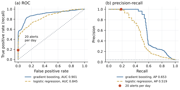
Figure 2.8. ROC curves (a) and precision-recall curves (b) of the gradient boosting detector and the logistic regression of Lab 2, trained on days 0 to 9 and tested on days 10 to 13. The dotted lines are random rankings (the diagonal in (a), the test base rate in (b)). The marker shows the operating point of the gradient boosting detector at an alert budget of 20 alerts per day. In (a) it lies on the vertical axis, because all 80 alerts are attacks and the false positive rate is zero. The precision of the gradient boosting detector falls steeply once its recall passes a little over one half, because the remaining attacks, mostly command-and-control beacons absent from training, score no higher than much of the normal traffic.
To see the base-rate effect on real scores, Lab 2 reweights the normal test records so that attacks make up 1% and 0.1% of the weighted test set. The true and false positive rates, and so the ROC curve, stay exactly the same. The AP of the gradient boosting detector falls from 0.653 at the actual base rate to 0.571 at 1% and 0.504 at 0.1%, as Figure 2.9 shows.
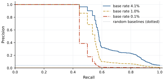
Figure 2.9. The precision-recall curve of the gradient boosting detector of Lab 2 at its actual test base rate and at two lower base rates, obtained by weighting the normal test records so that attacks make up 1% and 0.1% of the weighted total, which is equivalent to applying the Bayes-rule formula for precision of Lesson 1.2 to the same true and false positive rates. Its ROC curve is identical at all three base rates. Each dotted line is the corresponding random baseline. Precision at high recall collapses as attacks become rarer, because the same false positive rate is applied to more normal records per attack.
Choosing a threshold from an alert budget
A security operations team can investigate only so many alerts. If the budget is \(q\) alerts per day and the detector scores the traffic of \(D\) days, the threshold that exhausts the budget is the score of the \(k\)-th highest record, \(k = qD\). On the four test days of Lab 2, a budget of 20 alerts per day means 80 alerts. At that threshold the gradient boosting detector has a precision of 1.00 and a recall of 0.185. Every alert is a real attack, yet four in five attacks go unflagged. The budget, not the detector, limits the recall here, because the test days contain 432 attack records and the budget allows 80 alerts. Recall varies strongly by family. For example, 66% of denial-of-service records are flagged and 0% of the beacons.
That threshold was chosen by looking at the test days, which no deployed system can do. Lab 2 therefore also trains on days 0 to 7, sets the threshold so that days 8 and 9 together produce 40 alerts, 20 per day on average, and applies the fixed threshold to days 10 to 13. The detector then produces between 22 and 65 alerts per test day, over budget on every day, with a recall of 0.317 and a precision of 1.00. Every alert is an attack, so the overrun is caused by attacks above the threshold. The largest count, 65, falls on day 11, the only test day with denial-of-service traffic, and 43 of those alerts are denial-of-service records. A threshold fixes a score, not a number of alerts, and the number of records above it changes from day to day with the volume of attacks and of attack-like benign traffic. Arp et al. (2022) note a related difficulty for intrusion detection, where an operating point chosen from a ROC curve on test data can be hard to reproduce on the diversity of real traffic. In practice the alert count is monitored and the threshold revisited, or the detector is run in ranking mode, sending analysts the top \(q\) records each day whatever their scores.
Choosing a threshold from costs
Lesson 1.2 derived the decision rule of Elkan (2001). If a false alert costs \(c_{\mathrm{FP}}\), a missed attack costs \(c_{\mathrm{FN}}\), correct decisions cost nothing, and \(p\) is the probability that a record is an attack, alerting costs no more than staying quiet when \(p \ge c_{\mathrm{FP}}/(c_{\mathrm{FP}} + c_{\mathrm{FN}})\). If a missed attack costs fifty times as much as a false alert, the threshold is \(1/51 \approx 0.020\). The rule needs \(p\) to be a probability in the frequency sense, meaning that among records scored 0.02 about 2% must be attacks. A score that ranks well but is not calibrated gives the wrong operating point however good its AUC.
Calibration
A classifier is calibrated if, among the records to which it assigns probability \(p\), a share \(p\) are positive. A reliability diagram checks this. Niculescu-Mizil and Caruana (2005) describe the standard construction. Divide the predicted probabilities into ten bins of width 0.1, and for each bin plot the observed share of positives against the mean predicted probability. A calibrated model lies on the diagonal. The Brier score, the mean squared difference between the predicted probabilities of attack \(p_i\) and the labels \(y_i\) (1 for an attack, 0 for a normal record) over \(m\) records,
summarizes calibration and ranking together; lower is better.
Different models miscalibrate in characteristic ways. Niculescu-Mizil and Caruana found that maximum-margin methods such as support vector machines and boosted trees push predicted probabilities away from 0 and 1, producing a sigmoid-shaped reliability diagram, while naive Bayes pushes them toward 0 and 1. Two post-processing methods correct this. Platt scaling, introduced for support vector machines, fits a sigmoid \(p = 1/(1 + \exp(A f + B))\) to the model's score \(f\), with the two parameters \(A\) and \(B\) chosen by maximizing the likelihood of the labels. Isotonic regression fits an arbitrary nondecreasing step function from scores to probabilities. Isotonic regression can correct any monotone distortion, but Niculescu-Mizil and Caruana found it more prone to overfitting than Platt scaling when calibration data is scarce. Both must be fitted on data the model was not trained on; in scikit-learn, CalibratedClassifierCV does this by cross-validation, or on a held-out set when the trained model is wrapped in FrozenEstimator.
A common source of miscalibration in security is class weighting. With class_weight="balanced", scikit-learn weights each class by the inverse of its frequency, so the two classes contribute equally to the loss and the model is fitted as if the base rate were 0.5. A logistic regression trained this way estimates probabilities for a world in which half the records are attacks. Its ranking may be nearly unchanged, but its probabilities are far too high for the real base rate. Theorem 2 of Elkan (2001) gives the correction. If \(p\) is a correct probability for a population with base rate \(b\), the probability for the same record in a population with base rate \(b'\), assuming the class-conditional distributions are unchanged, is
For a balanced model, \(b = 0.5\). With a true base rate \(b' = 0.04\), an output of \(p = 0.5\) becomes \(p' = 0.04\), and an output of \(p = 0.9\) becomes
A balanced detector that is "90% sure" is right about a quarter of the time.
Lab 2 trains logistic regressions on days 0 to 7, recalibrates on days 8 and 9, and measures calibration on days 10 to 13, where 4.1% of records are attacks. Figure 2.10 shows the reliability diagrams, and the table below gives each model's mean predicted probability, Brier score and AP.
| Model | Mean predicted probability | Brier score | AP |
|---|---|---|---|
| Plain | 0.022 | 0.0261 | 0.523 |
| Balanced class weights | 0.081 | 0.0462 | 0.490 |
| Balanced, then Platt scaling | 0.016 | 0.0300 | 0.490 |
| Balanced, then isotonic regression | 0.017 | 0.0303 | 0.451 |
The table compares the four models on the test days. The balanced model's mean prediction is about twice the actual share of attacks and its Brier score is the worst. Both recalibrations bring the mean prediction down, close to the base rate of the calibration days, which is lower than that of the test days. Platt scaling is a monotone transformation and leaves the ranking, and therefore the AP, unchanged. Isotonic regression maps many different scores to the same value, and the resulting ties cost AP here. No calibration is perfect on the test days. The beacons that appear on day 10, absent from both the training and the calibration days, account for part of this, since almost all of their records fall in the lowest bin and raise the share of attacks there. The higher bins, which contain almost no beacons, also deviate from the diagonal, so a calibration fitted on days 8 and 9 does not carry over exactly to the test days. Calibration is a property of a model on a distribution, and it must be rechecked when the distribution drifts.
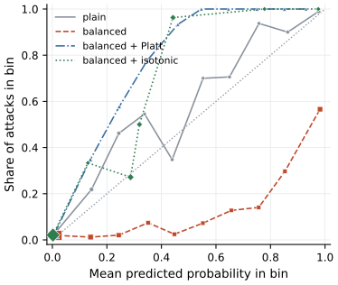
Figure 2.10. Reliability diagrams on the test days of Lab 2 for four logistic regressions trained on days 0 to 7. Each point is one bin of width 0.1 of predicted probability (bins with no records are omitted); its horizontal position is the mean predicted probability in the bin, its vertical position is the share of attacks among the records in it, and its area grows with the number of records in the bin. The dotted diagonal is perfect calibration. The balanced model lies below the diagonal (it overestimates the probability of attack). Platt scaling and isotonic regression were fitted on days 8 and 9, where attacks are rarer than on the test days, so the recalibrated models lie above the diagonal (they underestimate it).
Show the answer
With \(b = 0.5\), \(b' = 0.005\) and \(p = 0.7\), the numerator of equation \eqref{eq:elkan}, \(b'(p - p\,b)\), is \(0.005 \times 0.35\), or 0.00175. Its denominator, \(b - p\,b + b'\,p - b\,b'\), is \(0.5 - 0.35\) plus \(0.0035 - 0.0025\), or 0.151. So \(p' = 0.00175/0.151\), which is about 0.0116, or 1.2%. For the threshold, solve \(p' = 0.05\) for \(p\). Since \(p'\) increases with \(p\), you can search numerically or invert the formula. For \(b = 0.5\) it simplifies to
so the balanced odds must be
which is \(p \approx 0.913\). Only balanced outputs above about 0.91 justify an alert at that cost ratio.
What the lab shows
Lab 2
How leakage inflates a detector
Open in ColabRead with outputsNotebook on GitHubAbout 2 minutes to run on a laptop CPU
Sections 5 to 7 of Lab 2 produce the curves, the alert-budget thresholds and the reliability diagrams of this lesson. Try a budget of 5 alerts per day and see which families vanish from the alerts first.
Summary
A detector's score defines a family of operating points. The ROC curve and its area describe the ranking independently of the base rate, and the AUC is the probability that a random attack outscores a random normal record. The precision-recall curve and average precision describe what analysts experience at the actual base rate. AP is a step-wise sum, it equals about the base rate for a random ranking, and it cannot be compared across datasets with different attack shares. A threshold can be set from an alert budget, which must be fixed on past data and monitored as traffic drifts, or from the costs of errors, which requires calibrated probabilities. Reliability diagrams and the Brier score check calibration; Platt scaling and isotonic regression repair it on held-out data; and class weighting, convenient for training on rare attacks, inflates the odds of attack by a constant factor, which Elkan's formula undoes.
References
- Arp, D., Quiring, E., Pendlebury, F., Warnecke, A., Pierazzi, F., Wressnegger, C., Cavallaro, L., and Rieck, K. (2022). Dos and don'ts of machine learning in computer security. Proceedings of the 31st USENIX Security Symposium, 3971-3988. https://www.usenix.org/conference/usenixsecurity22/presentation/arp
- Davis, J., and Goadrich, M. (2006). The relationship between precision-recall and ROC curves. Proceedings of the 23rd International Conference on Machine Learning, 233-240. https://doi.org/10.1145/1143844.1143874
- Elkan, C. (2001). The foundations of cost-sensitive learning. Proceedings of the Seventeenth International Joint Conference on Artificial Intelligence (IJCAI), 973-978. https://www.ijcai.org/Proceedings/01/IJCAI-2001-k.pdf
- Fawcett, T. (2006). An introduction to ROC analysis. Pattern Recognition Letters, 27(8), 861-874. https://doi.org/10.1016/j.patrec.2005.10.010
- Niculescu-Mizil, A., and Caruana, R. (2005). Predicting good probabilities with supervised learning. Proceedings of the 22nd International Conference on Machine Learning, 625-632. https://doi.org/10.1145/1102351.1102430
- Saito, T., and Rehmsmeier, M. (2015). The precision-recall plot is more informative than the ROC plot when evaluating binary classifiers on imbalanced datasets. PLOS ONE, 10(3), e0118432. https://doi.org/10.1371/journal.pone.0118432