Unit 2 · Lesson 2.1
Preparing security data
A learning algorithm sees only a table of numbers. Everything between the raw evidence (packets, log lines, files, messages) and that table is a sequence of decisions, and most of them change what the model can learn. This lesson covers the decisions that matter most for security data, namely cleaning, missing values, categorical variables, scaling, skewed counts and text. One rule applies to all of them. A step that learns nothing from the data, such as dropping exact duplicates or taking a logarithm, can be done before the data is split. A step that learns something from the data, such as a median, a vocabulary or the attack rate of a category, must learn it from the training data only.
What security data looks like
Security problems produce several kinds of raw data, and each kind is usually turned into features in a characteristic way, as the table below summarizes.
| Kind of data | Examples | Typical features |
|---|---|---|
| Network flows | NetFlow or IPFIX records, connection logs | numeric counts, byte volumes, durations, rates over a time window, protocol and service as categories |
| Host and application logs | authentication logs, process creation events, web server logs | event counts per host and time window, categorical fields, sequences of event types |
| Binaries | executables, documents with macros | byte histograms, imported functions, section properties, strings |
| Text | e-mail bodies, command lines, scripts | token or character n-gram counts, TF-IDF weights, embeddings |
| URLs and domain names | links in e-mail, DNS queries | character n-grams, lengths, counts of digits and dots, top-level domain |
The course dataset flows.csv is of the first kind. Each row is one connection, with the source host (src_host), the office site, the categorical fields protocol and service, byte and packet volumes, counts and rates computed over recent connections, the number of failed logins, the time and the labels (Lesson 1.3 describes every column). The file urls.csv is of the last kind. Most of what follows applies to every kind.
Cleaning, and when it may happen
Cleaning removes records and values that do not describe the phenomenon you want to model, such as exact duplicates, records with impossible values (a negative byte count, a timestamp in the future), test traffic generated by the monitoring system itself, and inconsistent encodings of the same value (HTTPS, https, 443/tcp). Logs from different sources may use different time zones, so convert every timestamp to Coordinated Universal Time (UTC) before you sort, window or split by time.
Duplicated records are common in security data. Collectors retransmit, the same alert is forwarded by two sensors, and the same malware sample is submitted under many names. In the KDD Cup 1999 intrusion dataset, Tavallaee et al. (2009) found that about 78% of the training records and 75% of the test records were duplicates, which biased learners toward the frequent records and biased the evaluation toward methods that detect those records well. The course dataset has 1,103 exact duplicates, 2.9% of its rows.
Whether a row survives deduplication depends only on whether an identical row exists, not on any statistic, so deduplication may be done before the data is split. It should be, so that copies of a test record cannot sit in the training set (Lesson 2.2 measures what such copies do to a score). The same reasoning applies to any rule that looks at one record at a time, such as discarding rows with a negative duration.
A rule that depends on the whole dataset is different. Removing outliers defined as values more than three standard deviations from the mean uses a mean and a standard deviation, and if those are computed on all the data, the test set has shaped the training set. Arp et al. (2022) call this selective snooping, a form of data snooping, and give the removal of outliers based on statistics of the complete dataset as their example. Figure 2.1 shows where each kind of step belongs.
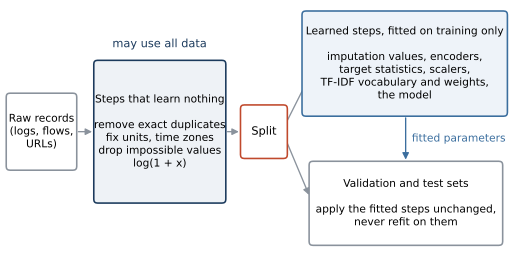
Figure 2.1. The order of data preparation. Steps on the left of the split learn nothing from the data (deduplication, fixing units and time zones, log transforms) and may be applied to all data. Steps on the right learn parameters from data (imputation values, encoder vocabularies and target statistics, scaling constants, TF-IDF weights, the model itself) and are fitted on the training set only, then applied unchanged to the validation and test sets.
In scikit-learn the simplest way to respect this order is to put every learned step inside a Pipeline or ColumnTransformer and to call fit only on training data. Cross-validation (Lesson 2.2) then refits the whole pipeline inside each fold automatically.
Missing values
Security data has gaps because a parser fails on a malformed packet, a field exists only for one protocol (an HTTP user agent has no meaning for a DNS query), a sensor is down for an hour, or an attacker deletes logs. The course dataset has no missing values, but real telemetry is rarely so complete.
You can drop rows with gaps, which is safe only when gaps are rare and unrelated to the label. You can impute, replacing each gap with a value such as the median of the column. Or you can use a model that handles missing values natively. In scikit-learn several tree-based classifiers, among them DecisionTreeClassifier, RandomForestClassifier and HistGradientBoostingClassifier, accept NaN directly (GradientBoostingClassifier does not). They learn at each split whether records with a missing value should go left or right, so missingness itself can carry information.
It often does. A connection without a server certificate, a process without a parent, or an e-mail without an authentication result can be suspicious because the field is empty. When you impute, an indicator column that is 1 where the value was missing preserves this signal,
import numpy as np
from sklearn.ensemble import HistGradientBoostingClassifier
from sklearn.impute import SimpleImputer

X = np.array([[1.0, 200.0], [np.nan, 3000.0],
              [0.5, np.nan], [2.0, 150.0]])
y = np.array([0, 1, 1, 0])
# NaN is accepted as is
HistGradientBoostingClassifier(max_iter=5).fit(X, y)

# in a real pipeline, fit on the training rows only
imp = SimpleImputer(strategy="median", add_indicator=True).fit(X)
print(imp.transform(X))
The imputer learns one median per column, so it belongs on the right of the split in Figure 2.1. Using the entire dataset for imputation is the first example that Kapoor and Narayanan (2023) give of leakage through pre-processing on the training and test sets.
Categorical variables
Fields such as protocol, service, site or a port number name categories. Their codes have no arithmetic meaning (port 443 is not "larger" than port 80 in any useful sense), so they must be encoded.
One-hot encoding creates one binary column per category. It assumes no order and suits linear models, distance-based models and neural networks. It becomes unwieldy when a field has thousands of values, such as a source address or a domain, and it cannot represent a category first seen after training (OneHotEncoder(handle_unknown="ignore") maps such a value to all zeros).
Ordinal encoding maps each category to an integer, which is appropriate when the categories have a real order, such as severity levels, but you must supply the order. By default OrdinalEncoder sorts the categories, which for strings means alphabetical order,
from sklearn.preprocessing import OrdinalEncoder
levels = [["low"], ["medium"], ["high"]]
print(OrdinalEncoder().fit(levels).categories_)
order = [["low", "medium", "high"]]
enc = OrdinalEncoder(categories=order).fit(levels)
print(enc.transform([["high"], ["low"]]))
The first print shows the order high, low, medium, which would tell a linear model that "low" lies between "high" and "medium". Tree models are less sensitive to an arbitrary integer code, because they can isolate a category with two splits, but they still waste splits on it.
Frequency encoding replaces each category by its share of the training records. It uses no labels, so it cannot leak them, although the shares are still learned and must come from the training data. It suits security data, where a service or user agent seen a few times in a month deserves attention.
Target encoding replaces each category by a statistic of the label within that category, typically the share of attacks. With \(n_c\) training records in category \(c\), of which \(s_c\) are attacks, and an overall attack share \(\bar y\), a smoothed estimate is
where \(m \ge 0\) controls how strongly a small category is pulled toward \(\bar y\). Target encoding packs the information of a high-cardinality field into one column, but it uses the label, and that creates a leak inside the training set itself. Consider eight training connections. The service is ssh for three of them (two attacks), http for four (one attack) and dns for one (normal), so \(\bar y = 3/8 = 0.375\). The table below gives, for each service, the number of records \(n_c\) and of attacks \(s_c\), the frequency encoding, the mean label \(s_c/n_c\) and the smoothed encoding \eqref{eq:target-encoding} with \(m = 2\).
| Service | \(n_c\) | \(s_c\) | Freq. | Mean | \(m = 2\) |
|---|---|---|---|---|---|
| ssh | 3 | 2 | 0.375 | 0.667 | 0.550 |
| http | 4 | 1 | 0.500 | 0.250 | 0.292 |
| dns | 1 | 0 | 0.125 | 0.000 | 0.250 |
In the table, the unsmoothed mean label of the dns row is exactly its own label. For any category with few records, the encoding computed on the training rows is largely a copy of their labels, so a flexible model learns to trust the column, and on new data, where the encoding no longer contains the record's own label, the trust is misplaced. Smoothing with \(m = 2\) moves the dns value to 0.25 but does not remove the dependence.
The remedy is cross-fitting. The training data is split into \(K\) folds, and each training row is encoded with statistics computed on the other \(K-1\) folds, so no row ever sees its own label. Scikit-learn's TargetEncoder does this in fit_transform by default, with five folds, while transform on new data uses statistics from the full training set. Calling fit and then transform on the training data skips the cross-fitting and reintroduces the leak.
Show the answer
The ssh category has three rows with labels 1, 1 and 0, so \(s_c = 2\) and \(n_c = 3\). A row with label 1 is encoded as \((2-1)/2 = 0.5\), and the row with label 0 as \((2-0)/2 = 1.0\). Within the category, the encoding of row \(i\) is a deterministic function of its own label \(y_i\) (1 for an attack, 0 for normal), namely \((s_c - y_i)/(n_c - 1)\), and the attacks receive the lower value. A tree can split on that difference and separate the training rows perfectly. Cross-fitting with \(K\) folds avoids this, because all rows of a category that fall in the same fold receive the same value, computed from the other folds, whatever their own labels.
Lab 2 measures the size of the effect. It adds to the flow features a synthetic identifier with 2,000 random values that carry no information about the label (about 13 training rows per value) and target-encodes it for a gradient boosting detector (Figure 2.2). Without the identifier the detector reaches an average precision (AP, defined in Lesson 2.3) of 0.654. With the naive encoding, fitted and applied on the same training rows, it falls to 0.256. With cross-fitting it is 0.649, unharmed, because the model learns that the column is useless. When the naive encoding is computed on all fourteen days before the split, the test rows are encoded with their own labels too, and the same useless column raises the test score to 0.751, a number that describes the leak and not the detector.
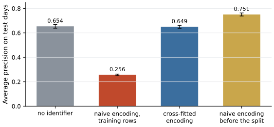
Figure 2.2. Average precision on the test days (days 10 to 13) of a gradient boosting detector trained on days 0 to 9, without and with a target-encoded synthetic identifier that carries no information about the label. Bars show the mean over five seeds and error bars one standard deviation. Naive encoding on the training rows destroys the detector; cross-fitting leaves it intact; naive encoding computed on all days inflates the test score. Data from Lab 2.
Scaling, and which models need it
Standardization maps each numeric feature \(x_j\) to \(z_j = (x_j - \mu_j)/\sigma_j\), where \(\mu_j\) and \(\sigma_j\) are the mean and standard deviation of feature \(j\) on the training data. Min-max scaling maps the training range to \([0, 1]\). Whether a model needs either depends on how it uses the features.
Models that compute distances between records, such as k-nearest neighbors, k-means clustering and support vector machines with a radial basis function kernel, need scaling, because otherwise the feature with the largest numeric range dominates every distance. In flows.csv, src_bytes reaches hundreds of millions while serror_rate lies between 0 and 1, so an unscaled Euclidean distance is essentially a difference in bytes. Regularized linear models need it because the penalty treats all coefficients alike. A feature with a small numeric range (bytes counted in gigabytes, say) needs a large coefficient to have the same effect as the same feature counted in bytes, and the penalty punishes that coefficient more. Principal component analysis needs it because a feature with a large range has a large variance and dominates the directions of maximal variance. Neural networks train faster and more reliably on inputs of similar scale. Tree ensembles, including random forests and gradient boosted trees, do not need scaling, because a split of the form \(x_j \le \theta\) at a threshold \(\theta\) depends only on the order of the values, and any increasing transformation of \(x_j\) leaves the order unchanged.
Lab 2 checks how much it matters to fit a scaler on all the data instead of on the training days. For a logistic regression the change in AP is +0.0004, which is negligible. A mean and a standard deviation estimated from 26,275 training rows barely move when 10,495 test rows are added, and a shift or rescaling of a feature affects a logistic regression only through its penalty. The rule stays the same, because the habit that is harmless for a scaler is harmful for the target encoder above, and a pipeline protects you from both.
Skewed features and the log transform
Volumes and counts in network data are heavy-tailed. Most connections transfer a few kilobytes, while backups and exfiltration move gigabytes. Figure 2.3 shows src_bytes in the course dataset on a linear and a logarithmic axis.
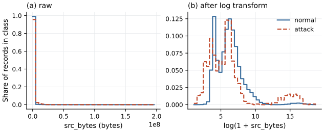
Figure 2.3. Distribution of src_bytes in flows.csv after deduplication, for normal connections (blue) and attacks (red), as the share of each class per bin. Left, the raw values, where almost every record falls into the first bin. Right, the values after the transform \(\log(1 + x)\), where the structure of both classes is visible, including the large uploads of backups and exfiltration on the right. Computed directly from the dataset.
A transform such as \(\log(1+x)\) compresses the tail, so that a distance or a linear coefficient reflects ratios instead of raw differences. This often helps linear, distance-based and neural models a great deal, and for trees it changes nothing, for the reason given above. The transform has no parameters learned from data, so it can be applied before the split.
Show the answer
No. Both transformations are strictly increasing in each feature, so every possible split \(x_j \le \theta\) on the raw data corresponds to a split on the transformed data that sends exactly the same records to each side, and the impurity of each candidate split is unchanged. With the same random seed the trees make the same choices. (In practice tiny differences can arise from floating-point ties and from how thresholds are placed between values, but not from the transformation itself.)
Text features for security
For command lines, scripts, e-mail bodies and URLs, the classical representation is a bag of words, a vector of counts with one entry per term in a vocabulary learned from the training documents. Term weighting refines it. Sparck Jones (1972) argued that matches on terms that occur in few documents should count for more than matches on frequent terms, and proposed weighting each term by a logarithmic function of its collection frequency. The resulting weight is known as inverse document frequency. In scikit-learn's default form, for a corpus of \(n\) training documents of which \(\mathrm{df}(t)\) contain term \(t\),
where \(\mathrm{tf}(t,d)\) is the number of times \(t\) occurs in document \(d\), and each document's vector \(w_{\cdot,d}\) is then divided by its Euclidean length. The added ones prevent division by zero and keep a term that occurs in every document from receiving zero weight.
Take three command lines as the training corpus,
powershell -nop -w hidden -enc SQBFAFgA
powershell -enc JABzAD0A
powershell Get-ChildItem -Path temp
and split them at whitespace. With \(n = 3\), the term powershell occurs in all three documents, so \(\mathrm{idf} = \ln(4/4) + 1 = 1\). The flag -enc occurs in two, so \(\mathrm{idf} = \ln(4/3) + 1 = 1.288\), and the encoded payload jabzad0a (lowercased) occurs in one, so \(\mathrm{idf} = \ln(4/2) + 1 = 1.693\). The second command line has the raw vector \((1, 1.288, 1.693)\) over these three terms, of Euclidean length 2.351, so after normalization its weights are 0.425, 0.548 and 0.720. The rare payload weighs most and the ubiquitous program name least.
How the text is cut into terms matters as much as the weights. Scikit-learn's default token pattern keeps runs of two or more letters, digits or underscores. Applied to the first command line, it returns enc, hidden, nop, powershell and sqbfafga. The leading hyphen of -enc is lost, so the flag becomes indistinguishable from the word "enc" anywhere else, and the single-letter flag -w disappears entirely. For command lines a custom pattern such as token_pattern=r"\S+" keeps the flags intact, and character n-grams (analyzer="char") go further,
from sklearn.feature_extraction.text import CountVectorizer
cmd = ["powershell -nop -w hidden -enc SQBFAFgA"]
print(CountVectorizer().fit(cmd).get_feature_names_out())
words = CountVectorizer(token_pattern=r"\S+").fit(cmd)
print(words.get_feature_names_out())
chars = CountVectorizer(analyzer="char", ngram_range=(3, 3)).fit(cmd)
print(chars.get_feature_names_out()[:8])
Character n-grams see fragments like -en and -w, survive small changes in spelling, case or obfuscation, and work on strings that have no natural word boundaries, such as URLs and domain names. Ma et al. (2009) classified URLs as malicious from bag-of-words tokens of the host name and path, split at punctuation, together with host-based features, and reported 95 to 99% accuracy on their data. Whether TF-IDF weights beat raw counts or binary presence depends on the model and the data (in short strings such as URLs most terms occur once), so the representation is a choice to evaluate on validation data. Lab 3b pairs each model with one weighting, TF-IDF weights for logistic regression and counts for naive Bayes, and compares word tokens with character n-grams for each model over five random 70/30 splits of the synthetic URLs of the course.
The vocabulary and the IDF weights are learned from the corpus, so they too belong on the right of Figure 2.1. Arp et al. (2022) note that computing TF-IDF weights or embeddings over the entire dataset is a common mistake that lets test documents shape the features.
Show the answer
First, the vocabulary was chosen with knowledge of the test set. It contains n-grams that occur only in test URLs, and with min_df or max_features the choice of which training n-grams survive also depends on test counts. Second, the IDF weights of all terms are computed from document frequencies that include the test URLs, so the scaling of every training feature depends on the test set. Neither uses the labels, so the effect is usually smaller than label leakage, but the evaluation is no longer of a model that saw only training data.
What the lab shows
Lab 2
How leakage inflates a detector
Open in ColabRead with outputsNotebook on GitHubAbout 2 minutes to run on a laptop CPU
Lab 2 removes the duplicated records before any split, keeps every learned step inside a pipeline, and then breaks these rules one at a time to measure what each violation does to the score.
Summary
Preparing security data means turning heterogeneous evidence into a table without letting the test data shape it. Steps that learn nothing from the data, such as deduplication, fixing units and time zones or taking a logarithm, can precede the split. Steps that learn from the data, from imputation values and encoder vocabularies to target statistics, scaling constants and TF-IDF weights, are fitted on training data only, which a pipeline enforces. Missingness can itself be informative. Target encoding needs cross-fitting. Scaling matters for distance-based, regularized linear and neural models but not for trees, and heavy-tailed counts benefit from a log transform. For command lines and URLs, the tokenizer decides what the model can see, which often argues for custom tokens or character n-grams.
References
- Arp, D., Quiring, E., Pendlebury, F., Warnecke, A., Pierazzi, F., Wressnegger, C., Cavallaro, L., and Rieck, K. (2022). Dos and don'ts of machine learning in computer security. Proceedings of the 31st USENIX Security Symposium, 3971-3988. https://www.usenix.org/conference/usenixsecurity22/presentation/arp
- Kapoor, S., and Narayanan, A. (2023). Leakage and the reproducibility crisis in machine-learning-based science. Patterns, 4(9), 100804. https://doi.org/10.1016/j.patter.2023.100804
- Ma, J., Saul, L. K., Savage, S., and Voelker, G. M. (2009). Beyond blacklists: Learning to detect malicious web sites from suspicious URLs. Proceedings of the 15th ACM SIGKDD International Conference on Knowledge Discovery and Data Mining, 1245-1254. https://doi.org/10.1145/1557019.1557153
- Sparck Jones, K. (1972). A statistical interpretation of term specificity and its application in retrieval. Journal of Documentation, 28(1), 11-21. https://doi.org/10.1108/eb026526
- Tavallaee, M., Bagheri, E., Lu, W., and Ghorbani, A. A. (2009). A detailed analysis of the KDD CUP 99 data set. 2009 IEEE Symposium on Computational Intelligence for Security and Defense Applications, 1-6. https://doi.org/10.1109/CISDA.2009.5356528