Unit 1 · Lesson 1.2
Base rates, metrics and the cost of an alert
A detector earns its place in a security team only if analysts can act on what it reports. Whether they can depends less on how often the detector is right than on how its mistakes are distributed, and that distribution is governed by a quantity the detector does not control, the base rate, which is the share of events that are actually attacks. This lesson defines the measures used throughout the course, shows why accuracy is almost useless when attacks are rare, and turns error rates into the number that matters operationally, the number of alerts an analyst must examine each day.
Four outcomes
Suppose a detector examines a stream of network connections and raises an alert on some of them. Every connection falls into one of the four cells of the table below, depending on whether it was an attack and whether the detector alerted.
| Detector alerts | Detector stays quiet | |
|---|---|---|
| Attack | true positive (TP) | false negative (FN) |
| Normal | false positive (FP) | true negative (TN) |
The table is called a confusion matrix. Every measure in this lesson is a ratio of its cells. Two of them describe the detector's behavior on each class separately. The true positive rate, also called recall or detection rate, is the share of attacks that raise an alert, and the false positive rate, also called the false alarm rate, is the share of normal connections that raise an alert. In terms of the four counts,
Two further measures describe the alerts and the overall result. Precision is the share of alerts that are real attacks, and accuracy is the share of all connections classified correctly,
The F1 score combines precision and recall into one number through their harmonic mean,
It is convenient for ranking models, but it hides which of the two is weak, so this course reports precision and recall separately whenever the difference matters.
Recall and the false positive rate each look at one class only. Precision and accuracy mix the two classes, so in general they change when the mix changes. That distinction is the subject of the rest of the lesson.
A detector that catches almost everything
Consider a detector with a true positive rate of 0.99 and a false positive rate of 0.01, applied to 100,000 connections of which 0.1%, or 100, are attacks. It detects 99 of the 100 attacks and misses one. Of the 99,900 normal connections, 1% or 999 raise an alert, and 98,901 do not. Figure 1.3 draws these counts as a tree.
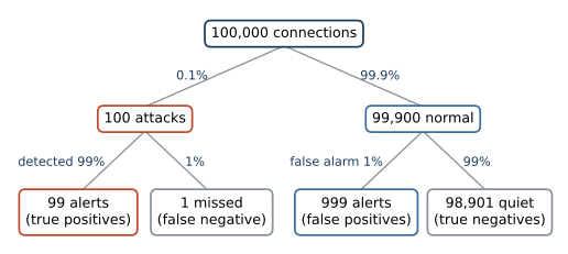
Figure 1.3. The detector of the worked example applied to 100,000 connections with a base rate of 0.1%. Each branch is labeled with the share of its parent that follows it, and each leaf gives the resulting number of connections. Of the 1,098 alerts at the bottom, 99 are real.
The detector raises 1,098 alerts, and 99 of them are real, so its precision is \(99/1{,}098 \approx 0.090\). An analyst who investigates every alert finds an attack about once in eleven attempts, and spends the other ten on benign traffic. Its accuracy is \((99 + 98{,}901)/100{,}000\), or 0.990, and its F1 score is about 0.165.
Now consider a detector that never raises an alert. It classifies all 99,900 normal connections correctly and misses all 100 attacks, so its accuracy is \(99{,}900/100{,}000 = 0.999\), higher than that of the first detector. Its recall is zero. Its precision is undefined, because it raises no alerts and the fraction in \eqref{eq:prec-acc} is \(0/0\). (Scikit-learn reports zero in that case and issues a warning; the argument zero_division controls the value.)
A detector that never fires beats one that catches 99% of attacks on accuracy. When one class is rare, accuracy mostly measures how well a detector handles the common class, which is rarely where the difficulty lies. For that reason this course does not use accuracy to evaluate detectors of rare attacks. Accuracy appears mainly where the classes are roughly balanced, as for the image classifiers of Units 6 to 8.
Show the answer
TPR and FPR would not change, because each is computed within one class. Precision would rise, because there would be ten times as many true positives against roughly the same number of false positives. With 1,000 attacks and 99,000 normal connections, the detector raises 990 true and 990 false alerts, so precision becomes 0.5. Accuracy is \((990 + 98{,}010)/100{,}000\), still 0.990, but only because the detector happens to make errors at the same rate on both classes (1% of attacks missed and 1% of normal connections flagged). Accuracy is the average of the per-class accuracies weighted by the class shares, so in general it moves when the shares move.
Bayes' rule and the base-rate fallacy
Let \(\pi\) denote the base rate, the probability that a randomly chosen connection is an attack. Precision is the probability that a connection is an attack given that it raised an alert. Bayes' rule expresses it through the two class-wise rates and the base rate,
The numerator counts true alerts and the denominator counts all alerts, both as fractions of all connections. With \(\pi = 0.001\), \(\mathrm{TPR} = 0.99\) and \(\mathrm{FPR} = 0.01\), the numerator of \eqref{eq:bayes} is \(0.00099\) and the denominator is \(0.00099 + 0.00999\), so the ratio is about 0.090, the precision of the worked example.
When \(\pi\) is small, the term \(\mathrm{FPR}\,(1-\pi)\) dominates the denominator unless the false positive rate is smaller still. For precision to reach one half, true alerts must at least equal false ones, \(\mathrm{TPR}\,\pi \ge \mathrm{FPR}\,(1-\pi)\), which requires
In words, the false positive rate has to be about as small as the base rate itself. Improving recall helps little. Raising the true positive rate from 0.5 to 1 only doubles the numerator of \eqref{eq:bayes}, while the false positive rate may need to fall by several orders of magnitude. Figure 1.4 plots equation \eqref{eq:bayes} for a fixed true positive rate and four false positive rates.
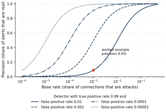
Figure 1.4. Precision from equation \eqref{eq:bayes} as a function of the base rate, for a detector with a true positive rate of 0.99 and four false positive rates. The base-rate axis is logarithmic. The marked point is the worked example, a base rate of 0.1% and a false positive rate of 0.01, which gives a precision of 9.0%. Each tenfold reduction in the false positive rate shifts the curve about tenfold to the left.
Ignoring the base rate when judging a test result is a reasoning error known as the base-rate fallacy. Axelsson (2000) showed what it implies for intrusion detection. He considered a hypothetical installation that produces about one million audit records a day and suffers one or two intrusions a day, each touching about ten records. Taking two intrusions a day, as Axelsson does, gives a base rate of \(2 \times 10^{-5}\). Even a detector that caught every intrusion would need a false alarm rate on the order of \(10^{-5}\) for two thirds of its alarms to be real, and with a detection rate of 0.7 the same false alarm rate gives about 58%. You can check both figures with equation \eqref{eq:bayes}. Two decades later, Arp et al. (2022) still list the base-rate fallacy among ten common pitfalls in machine learning for security, describing it as the misinterpretation of performance when a large class imbalance is ignored.
The cost of an alert
Rates become workload once they are multiplied by traffic volume. A network that carries one million benign connections a day and a detector with a false positive rate of 0.001 together produce about 1,000 false alerts a day, before a single attack occurs. If one analyst can investigate, say, a few dozen alerts in a shift, that detector is unusable however good its recall. Sommer and Paxson (2010) observe that the relative cost of a misclassification in intrusion detection is extremely high compared with many other applications of machine learning. A false positive consumes analyst time on benign activity, and a false negative can leave a compromised system in place.
This suggests two ways to choose how a detector should operate. The first fixes an alert budget, the number of alerts the team can investigate per day, and sets the detector's threshold so that it does not exceed the budget. Lesson 2.3 develops this approach. The second assigns a cost to each kind of error. Let \(c_{\mathrm{FP}}\) be the cost of investigating a false alert and \(c_{\mathrm{FN}}\) the cost of missing an attack, with correct decisions costing nothing. If a model outputs a calibrated probability \(p\) that a connection is an attack, raising an alert has expected cost \((1-p)\,c_{\mathrm{FP}}\) and staying quiet has expected cost \(p\,c_{\mathrm{FN}}\). Alerting costs no more than staying quiet when
which is a special case of the optimal decision threshold derived by Elkan (2001). If a missed attack costs 99 times as much as a false alert, the threshold is 0.01, far below the default of 0.5 that most libraries apply. The rule holds only when the probabilities are calibrated, meaning that among connections given probability 0.2 about 20% really are attacks. Lesson 2.3 shows how to check calibration.
Show the answer
From equation \eqref{eq:fpr-bound}, \(\mathrm{FPR} \le \mathrm{TPR}\,\pi/(1-\pi)\). With \(\mathrm{TPR} = 0.9\) and \(\pi = 10^{-4}\), the bound is \(0.9 \times 10^{-4}/0.9999\), or about \(9 \times 10^{-5}\). The detector may raise a false alert on at most about one normal connection in 11,000.
What the lab shows
Lab 1
A first look at the network data
Open in ColabRead with outputsNotebook on GitHubAbout 1 minute to run on a laptop CPU
In Lab 1 you load the course dataset, in which 1,066 of 37,873 connection records are attacks, and train a logistic regression on the first ten days. On the last four days, a detector that never alerts is 95.9% accurate, and the trained model reaches 97.1%, a difference that says almost nothing about either. The model's recall at the default threshold is 0.31 and its precision is 0.95, so most of its alerts are real but most attacks go unnoticed. It detects none of the command-and-control traffic that first appears in the test days. Applying equation \eqref{eq:bayes} to its error rates shows that at a base rate of 0.1% its precision would fall to 0.29.
Summary
Recall and the false positive rate describe a detector and do not depend on the base rate. Precision and accuracy also depend on how common attacks are, and when attacks are rare, accuracy is dominated by the normal class and precision is dominated by the false positive rate. A useful detector for a rare attack needs a false positive rate comparable to the base rate, and its threshold should be set from the cost of errors or from the alert budget of the people who will read its output.
References
- Arp, D., Quiring, E., Pendlebury, F., Warnecke, A., Pierazzi, F., Wressnegger, C., Cavallaro, L., and Rieck, K. (2022). Dos and don'ts of machine learning in computer security. Proceedings of the 31st USENIX Security Symposium, 3971-3988. https://www.usenix.org/conference/usenixsecurity22/presentation/arp
- Axelsson, S. (2000). The base-rate fallacy and the difficulty of intrusion detection. ACM Transactions on Information and System Security, 3(3), 186-205. https://doi.org/10.1145/357830.357849
- Elkan, C. (2001). The foundations of cost-sensitive learning. Proceedings of the Seventeenth International Joint Conference on Artificial Intelligence (IJCAI), 973-978. https://www.ijcai.org/Proceedings/01/IJCAI-2001-k.pdf
- Sommer, R., and Paxson, V. (2010). Outside the closed world: On using machine learning for network intrusion detection. 2010 IEEE Symposium on Security and Privacy, 305-316. https://doi.org/10.1109/SP.2010.25