Unit 1 · Lesson 1.3
The workflow, the tools and the course dataset
A detector is the end product of a sequence of decisions, and most of the ways a security model fails are set in that sequence before any algorithm is chosen. This lesson walks through the workflow from framing the problem to retraining a deployed model, explains what it takes for a result to be reproducible, introduces the software used in the labs, and describes the synthetic dataset that eight of the labs share. It ends with the public datasets that dominate the research literature and the problems that have been documented in them.
The workflow
Figure 1.5 shows the stages as a loop. Each stage is described below with the mistake that is most typical of it in security work.
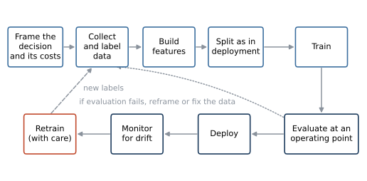
Figure 1.5. The workflow for building a detector. The top row prepares the data and the model, and the bottom row runs it. A failed evaluation sends the work back to framing or to the data (dotted arrow), and retraining returns to data collection with the labels gathered in operation (dashed arrow). Retraining is marked in red because it is where drift is corrected and also where poisoned labels can enter.
Framing the decision comes first. Who acts on the output, what does an alert cost them, what does a missed attack cost, and how many alerts can they investigate in a day? The answers fix the performance measure and the operating point before any data is touched. A detector for an analyst team with an alert budget of 50 a day is judged by its recall within those 50 alerts; Lesson 1.2 showed why accuracy cannot stand in for that.
Data collection and labeling come next. The data must contain the events the detector will see in deployment, with labels that mean what you think they mean. Labels in security usually come from analysts, from external services or from heuristics, and each source has its own errors (Lesson 1.1). Labels also arrive late, often after an investigation, which matters for the leakage problem described below.
Feature construction turns raw events into the vectors \(x\) of Lesson 1.1. The rule that governs it is simple to state and easy to break. A feature may use only information that exists at the moment the detector has to decide.
Splitting must mirror deployment. A detector is trained on the past and applied to the future, so the test set should come after the training set in time. With \(x_i\) and \(y_i\) the features and label of event \(i\), \(t_i\) its time and \(\tau\) a cut-off time,
A random split instead mixes future events into training, which Arp et al. (2022) call temporal snooping and Pendlebury et al. (2019) call temporal bias. If the detector will serve a site it was not trained on, the split should also hold out sites, and if records repeat, every copy of a record should fall on the same side of the split. Unit 2 develops these rules.
Training fits the model on the training set, and any choice of hyperparameters or threshold is made on a validation set carved from the training period, never on the test set.
Evaluation takes place at an operating point. A detector that outputs scores has no single error rate until a threshold is chosen, so it is evaluated at the threshold it will actually use, chosen from the alert budget or from the costs of Lesson 1.2, along with curves that show the alternatives (Lesson 2.3).
Deployment exposes the detector to traffic it has not seen, and its operating point translates into a daily workload. If a site carries \(N\) events a day with base rate \(\pi\), a detector with true positive rate \(\mathrm{TPR}\) and false positive rate \(\mathrm{FPR}\) raises on average
alerts a day.
Monitoring checks whether that expectation still holds. A sudden change in the number of alerts, in the mix of services, or in the distribution of scores is often the first visible sign of drift, of a new attack, or of a broken data feed. If alerts arrive independently, the daily count is approximately Poisson with mean \(\mu\) and standard deviation \(\sqrt{\mu}\), and a simple check standardizes the observed count \(A\),
As a worked example, take \(N = 50{,}000\) connections a day, \(\pi = 0.002\), \(\mathrm{TPR} = 0.8\) and \(\mathrm{FPR} = 0.001\). Equation \eqref{eq:expected-alerts} gives \(50{,}000 \times 0.998 \times 0.001 = 49.9\) false alerts and \(50{,}000 \times 0.002 \times 0.8 = 80\) true alerts, so \(\mu = 129.9\) and \(\sqrt{\mu} \approx 11.4\). A day with 200 alerts gives \(z \approx 6.2\) by \eqref{eq:alert-z}, far outside ordinary variation, while a day with 150 gives \(z \approx 1.8\), which is unremarkable on its own. Alerts are rarely independent in practice, since one noisy host can produce many, so the Poisson model usually understates the day-to-day variation. A practical monitor compares each day with the recent history of the same site and weekday.
Retraining corrects drift, and it carries risks of its own. New labels come mostly from alerts that analysts examined, so events the old model ignored are underrepresented, and a model retrained on them can inherit its predecessor's blind spots. Labels that reach the training set without review are also an entry point for poisoning (Lesson 1.1). A retrained model should pass the same time-ordered evaluation as the original before it replaces it.
Show the answer
False alerts become \(50{,}000 \times 0.996 \times 0.001 = 49.8\) and true alerts \(50{,}000 \times 0.004 \times 0.8 = 160\), so \(\mu = 209.8\). Against the old mean, \(z = (209.8 - 129.9)/\sqrt{129.9} \approx 7.0\). The monitor would notice the campaign through the alert count alone, even before anyone looked at the alerts.
Reproducibility
A result is reproducible when someone else can obtain the same numbers from the same inputs. A notebook that runs from top to bottom without errors is not enough, because four things can still change between two runs. The first is randomness. Random splits, weight initialization and sampling all draw on a pseudo-random generator, and the labs fix its seed explicitly, with numpy.random.default_rng(seed) for NumPy, random_state= for scikit-learn and torch.manual_seed(seed) for PyTorch. Mixing the legacy global function np.random.seed with generator objects makes it hard to tell which stream a result came from, so the course uses generator objects only. The second is the software. A new release of a library can change a default argument or a numerical routine, so the course pins the exact version of every package in requirements.txt. The third is the data, which must be versioned so that "the dataset" means one specific file. The course dataset is produced by a script with a fixed seed, and running it again reproduces the shipped file byte for byte. The fourth is the record of results. Every lab writes the numbers it reports to a file in labs/results/, and the lessons quote those files, so a number in the text cannot drift away from the code that produced it.
The tools
The labs are written in Python 3.12 and use a small set of libraries: NumPy for arrays and random numbers, pandas for tables, scikit-learn for classical models, pipelines and metrics, PyTorch for neural networks, and Matplotlib for plots. Some labs also use torchvision for image data, Hugging Face transformers for pretrained language models, and Opacus for privacy accounting in differentially private training. Every lab runs on a laptop CPU without a GPU, and each lab card states roughly how many minutes it takes. You can run the labs in Google Colab, which needs only a free Google account and has all of these libraries except Opacus preinstalled (the differential-privacy lab installs Opacus in its first cell), or locally in a virtual environment built from requirements.txt. Colab's library versions differ from the pinned ones, so results there may differ in the last digits from those printed in the lessons. The Python primer covers what you need of NumPy, pandas, Matplotlib and scikit-learn; PyTorch and the other libraries are introduced in the units that use them, from Unit 5 on.
The course dataset
Eight of the nineteen labs use one synthetic dataset, data/flows.csv, generated by data/make_dataset.py. It contains 37,873 records of network connections from two office sites over 14 days, from 2025-03-03T00:03:05Z to 2025-03-16T23:59:51Z (times in UTC). No record describes a real network, host or person. Each row is one connection record and has the 21 columns listed in Table 1.2.
| Column | Meaning |
|---|---|
timestamp |
start of the connection, UTC, to the second |
day, hour |
day of the capture (0 to 13) and hour of the day (0 to 23) |
site |
A (main office) or B (branch office) |
src_host |
internal host that opened the connection, A001 to A140 or B001 to B060 |
protocol, service |
transport protocol (tcp or udp) and application service (http, https, dns, ssh, ftp, smtp, rdp or other) |
duration |
length of the connection in seconds |
src_bytes, dst_bytes |
bytes sent by the source and bytes returned by the destination |
packets |
packets in both directions |
failed_logins |
failed login attempts within the connection |
count, srv_count |
connections from the same source to the same destination host, and to the same service, in a recent window |
serror_rate, rerror_rate |
share of those connections with connection-setup errors and with rejected connections |
same_srv_rate |
share of those connections that used the same service |
dst_host_count |
distinct destination hosts the source contacted in a recent window |
ticket_opened |
1 if an analyst later opened a ticket for the connection |
attack_type |
normal, scan, bruteforce, dos, exfil or c2beacon |
label |
1 for an attack, 0 for normal |
Table 1.2. The columns of data/flows.csv. The window-based columns follow the style of the features in the KDD Cup 99 data (described at the end of this lesson), but the generator draws them from distributions chosen for each kind of behavior instead of computing them from a packet trace.
Site A, the main office, has 140 hosts and 25,512 records, of which 504 are attacks (2.0%). Site B, the branch office, is smaller, with weaker patching and more remote administration, and has 60 hosts and 12,361 records, of which 562 are attacks (4.5%). The base rate therefore differs between sites, which Unit 11 uses to audit a detector for unequal error rates. Overall, 2.8% of records are attacks, from the five families in Table 1.3. The scan family imitates probing of many hosts and ports, bruteforce password guessing over ssh, ftp and rdp, dos floods of short connections, exfil large uploads of stolen data, and c2beacon small, regular check-ins with a command-and-control server.
| Family | Records | Days present | Share at site B |
|---|---|---|---|
scan |
338 | 14 | 51% |
bruteforce |
266 | 14 | 61% |
dos |
165 | 3 | 47% |
exfil |
112 | 14 | 51% |
c2beacon |
185 | 4 | 51% |
Table 1.3. Attack families in the course dataset, counted by Lab 1. Records include duplicates. Days present is the number of distinct days on which the family occurs, out of 14. Share at site B is the fraction of the family's records that come from site B.
Figure 1.6 shows when the attacks occur. Scanning, brute force and exfiltration appear every day, denial of service occurs in bursts on 3 days, and the beaconing family first appears on day 10. A detector trained on the first ten days, as in Lab 1, has never seen a beacon, and Lab 1 shows that its recall on them is 0.00. This is the dataset's built-in example of drift.
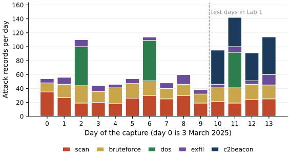
Figure 1.6. Attack records per day in the course dataset, stacked by family, as counted in Lab 1. Day 0 is 3 March 2025. Denial-of-service records occur on days 2, 6 and 11 only, and command-and-control beacons (dark blue) appear from day 10. The dashed line separates the ten training days from the four test days used in Lab 1.
The generator makes the two classes overlap. A share of each attack family is stealthy, with its numeric features blended toward the benign behavior it imitates. Four benign behaviors resemble attacks, and Lab 1 counts them with a simple rule each. Administrators who mistype their passwords produce 432 normal records with failed logins, beside 235 attack records with failed logins. Nightly backups produce 462 normal records that upload more than 100,000 bytes at night, while 112 attack records, all of them exfiltration, upload more than 100,000 bytes at various hours. The IT team's authorized vulnerability scanner, host A010, produces 169 records on days 3 and 9 that look like a port scan. A misconfigured service that keeps retrying a closed port produces 232 records with many rejected connections and no reply bytes, which resemble a denial-of-service flood. Figure 1.7 shows the resulting overlap on two features.
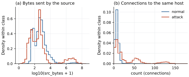
Figure 1.7. Distributions of two features for normal records (blue) and attack records (red), as computed in Lab 1, each normalized to unit area within its class. (a) Bytes sent by the source on a logarithmic scale; in the small peaks above about \(10^5\) bytes, the attack records are exfiltration and the normal records are mostly nightly backups. (b) Connections from the same source to the same host in a recent window. Most attack records fall within the range of normal traffic on both features, and the attack modes near 50 and 120 connections come from scanning and denial of service.
Two further properties are deliberate traps. Some records were logged twice, as happens when a collector retransmits. Lab 1 finds 1,103 exact duplicates (2.9% of records), 26 of them attacks. A random split puts copies of the same record on both sides, so the model is tested on records it has already seen. The column ticket_opened is the second trap. It is filled in after an analyst has investigated, and an analyst opened a ticket for 86% of attack records and 1% of normal ones. A model given this column would look excellent and be useless, because the column does not exist at the moment of decision. This is target leakage, and Unit 2 shows how much leakage can inflate a detector.
Show the answer
Under a random split each duplicated pair has a good chance of being separated, so the test set contains records whose exact copies were in training. A flexible model, such as a nearest-neighbor classifier or a deep tree, can memorize those records instead of generalizing, which inflates test performance. The inflation grows with the share of duplicates and when they are concentrated in the attack class. Here only 26 of the duplicates are attacks, and in Lesson 2.2 the effect of a similar share of duplicates on the detector's score is too small to measure. In this dataset the two copies share the same timestamp, so a split by time keeps them on the same side. Removing duplicates before splitting is still good practice.
A synthetic dataset has clear advantages for a course. Its ground truth is known exactly, since the generator decides what each record is. It contains no personal data, is released under the permissive MIT License, and is small enough to run on a laptop. It can be built to contain the problems a course needs to teach, such as look-alikes, drift, duplicates and a leaked column. It also has limits that you should keep in mind. Its features are drawn independently for each record from distributions the generator chose, so relationships between connections, payloads and the long tails of real traffic are absent. Its base rate of 2.8% is far higher than most networks would show, and its attacks are whatever the generator says they are. Results on it show how methods behave and fail. They do not show how a detector would perform on a real network.
Public datasets and their documented problems
Research on learned intrusion detection has relied on a small number of public datasets, and Tavallaee et al. (2009) describe KDD Cup 99 as the most widely used data set for evaluating anomaly detection systems. Sommer and Paxson (2010) explain why so few datasets exist. Network traffic reveals confidential and personal information, so organizations rarely release it, and researchers have fallen back on simulated traffic and on anonymized captures, both with serious limits. The best-known datasets have been examined closely, and the findings are a catalog of what can go wrong.
The DARPA intrusion detection evaluations of 1998 and 1999, run by MIT Lincoln Laboratory, produced weeks of traffic from a simulated network into which attacks were injected. McHugh (2000) criticized the design. For privacy reasons both the background traffic and the attacks were synthesized. As far as McHugh could determine from the published record, neither the false alarm characteristics of the artificial background nor the realism of the way attacks were distributed within it was validated. The KDD Cup 99 dataset distilled the 1998 traces into connection records with features such as those of Table 1.2. Tavallaee et al. (2009) found that about 78% of the training records and 75% of the test records were duplicates, and that 80% of the training records were attacks. When they labeled every record with 21 classifiers, about 98% of training records and 86% of test records were classified correctly by all 21. Easy records dominate, so the accuracies of different methods fall in a narrow band between about 86% and 100% and are hard to compare. Their NSL-KDD dataset removes the duplicates and selects records by difficulty, but the authors state that it still suffers from some of McHugh's problems and may not be a perfect representative of existing real networks.
CICIDS2017 was built to replace these older datasets. Sharafaldin et al. (2018) recorded five consecutive days, from Monday 3 July to Friday 7 July 2017, on a testbed whose benign traffic was generated from profiles of 25 users, and executed brute-force, denial-of-service, Heartbleed, web, infiltration, botnet and distributed denial-of-service attacks, extracting more than 80 flow features per connection. Engelen et al. (2021) reanalyzed the raw captures and found problems in traffic generation, flow construction, feature extraction and labeling. Labels had been assigned from attacker and victim addresses and a time window, so a flow was marked malicious simply for occurring between the two at the time of an attack, whether or not it carried any attack content. More than 25% of all flows were meaningless artifacts, reaching 50% for several attack categories, and after their corrections more than 20% of the original traffic traces were reconstructed or relabeled. UNSW-NB15 was generated in the Cyber Range Lab of UNSW Canberra with the IXIA PerfectStorm tool, as a hybrid of real normal activity and synthetic attacks of nine types, and contains about 2.5 million records (UNSW Canberra, n.d.).
Malware detection has a different kind of benchmark. EMBER (Anderson and Roth, 2018) provides features extracted from 1.1 million Windows executables, 900,000 for training (300,000 malicious, 300,000 benign and 300,000 unlabeled) and 200,000 for testing, with the test files first seen in the last two months of 2017, after the training files. Its labels come from antivirus vendors. A file labeled benign was flagged by no vendor and a file labeled malicious by more than 40, and the authors note that this makes EMBER a relatively easy dataset. Its test set is half malware, so a precision measured on it holds only at that base rate (Lesson 1.2).
These datasets remain useful for comparing methods under fixed conditions. None of them is a sample of a real deployment, and a result on any of them should be read with its documented problems and its base rate in mind. Arp et al. (2022) found sampling bias, data that do not represent the true distribution of the security problem, at least partly present in 90% of the papers they studied.
Show the answer
First, about 78% of the training records are duplicates, so a random split of the training file places copies of most test records in the training set, and the test largely measures memorization of records already seen in training. Second, about 98% of training records were classified correctly by all 21 of Tavallaee et al.'s learners, so almost any method reaches high accuracy on a random part of the training file; the comparison cannot separate good methods from weak ones. A third reason follows from Lesson 1.2. Attacks are about 80% of the training records, so accuracy says nothing about precision at a realistic base rate.
Lab 1 computes every number quoted above about the course dataset, and its last section is a short tour of the dataset that you can extend.
Lab 1
A first look at the network data
Open in ColabRead with outputsNotebook on GitHubAbout 1 minute to run on a laptop CPU
Summary
A detector is built in a loop that runs from framing the decision and its costs, through data, features, a split that mirrors deployment, training and evaluation at an operating point, to deployment, monitoring and retraining. Expected alert counts follow from the base rate and the error rates, and a simple Poisson check on daily counts gives early warning of drift. Reproducibility needs fixed seeds, pinned package versions, versioned data and recorded results. The course dataset is synthetic, with two sites, five attack families, a family that appears only in the last four days, benign look-alikes, duplicated records and a leaked column, so that each of these problems can be studied with known ground truth. Public benchmark datasets are convenient for comparison, but none is a sample of a real deployment, and the best-studied of them have documented flaws in realism, duplication or labeling that limit what results on them can show.
References
- Anderson, H. S., and Roth, P. (2018). EMBER: An open dataset for training static PE malware machine learning models. arXiv preprint arXiv:1804.04637. https://arxiv.org/abs/1804.04637
- Arp, D., Quiring, E., Pendlebury, F., Warnecke, A., Pierazzi, F., Wressnegger, C., Cavallaro, L., and Rieck, K. (2022). Dos and don'ts of machine learning in computer security. Proceedings of the 31st USENIX Security Symposium, 3971-3988. https://www.usenix.org/conference/usenixsecurity22/presentation/arp
- Engelen, G., Rimmer, V., and Joosen, W. (2021). Troubleshooting an intrusion detection dataset: The CICIDS2017 case study. 2021 IEEE Security and Privacy Workshops (SPW), 7-12. https://doi.org/10.1109/SPW53761.2021.00009
- McHugh, J. (2000). Testing intrusion detection systems: A critique of the 1998 and 1999 DARPA intrusion detection system evaluations as performed by Lincoln Laboratory. ACM Transactions on Information and System Security, 3(4), 262-294. https://doi.org/10.1145/382912.382923
- Pendlebury, F., Pierazzi, F., Jordaney, R., Kinder, J., and Cavallaro, L. (2019). TESSERACT: Eliminating experimental bias in malware classification across space and time. Proceedings of the 28th USENIX Security Symposium, 729-746. https://www.usenix.org/conference/usenixsecurity19/presentation/pendlebury
- Sharafaldin, I., Habibi Lashkari, A., and Ghorbani, A. A. (2018). Toward generating a new intrusion detection dataset and intrusion traffic characterization. Proceedings of the 4th International Conference on Information Systems Security and Privacy (ICISSP), 108-116. https://doi.org/10.5220/0006639801080116
- Sommer, R., and Paxson, V. (2010). Outside the closed world: On using machine learning for network intrusion detection. 2010 IEEE Symposium on Security and Privacy, 305-316. https://doi.org/10.1109/SP.2010.25
- Tavallaee, M., Bagheri, E., Lu, W., and Ghorbani, A. A. (2009). A detailed analysis of the KDD CUP 99 data set. 2009 IEEE Symposium on Computational Intelligence for Security and Defense Applications, 1-6. https://doi.org/10.1109/CISDA.2009.5356528
- UNSW Canberra (n.d.). The UNSW-NB15 dataset. Dataset page of the Cyber Range Lab, UNSW Canberra at ADFA, accessed 15 October 2026. https://research.unsw.edu.au/projects/unsw-nb15-dataset