Unit 1 · Lab 1
A first look at the network data
Lab 1
A first look at the network data
Open in ColabRead with outputsNotebook on GitHubAbout 1 minute to run on a laptop CPU
# On Google Colab, install the scikit-learn version the course was built with.
# On your own computer, install requirements.txt instead; this cell then does nothing.
import subprocess, sys
if "google.colab" in sys.modules:
    subprocess.run([sys.executable, "-m", "pip", "install", "-q", "scikit-learn==1.9.0"], check=True)
Lab 1. A first look at the network data
This lab introduces the dataset used in most of the course and shows, with a real model, why accuracy says little about a detector when attacks are rare. It runs in under a minute on a laptop CPU.
You will:
- load the connection records and see how rare the attacks are;
- score a detector that never raises an alert;
- train a logistic regression on the first ten days and test it on the last four;
- turn its error rates into alerts per day and into precision at a lower base rate;
- count what the dataset contains: sites, attack families, duplicates, a leaked column and benign look-alikes.
The data is synthetic. It was generated by data/make_dataset.py to behave like connection logs from two office sites, including benign activity that resembles attacks. Lesson 1.3 describes it in detail.
import os

import numpy as np
import pandas as pd
import matplotlib.pyplot as plt

from sklearn.compose import ColumnTransformer
from sklearn.linear_model import LogisticRegression
from sklearn.metrics import confusion_matrix
from sklearn.pipeline import make_pipeline
from sklearn.preprocessing import FunctionTransformer, OneHotEncoder, StandardScaler

LOCAL = "../../data/flows.csv"
URL = "https://raw.githubusercontent.com/aalbata/machine-learning-for-cybersecurity/main/data/flows.csv"
flows = pd.read_csv(LOCAL if os.path.exists(LOCAL) else URL)
print(flows.shape)
flows.head()
(37873, 21)
| timestamp | day | hour | site | src_host | protocol | service | duration | src_bytes | dst_bytes | ... | failed_logins | count | srv_count | serror_rate | rerror_rate | same_srv_rate | dst_host_count | ticket_opened | attack_type | label | |
|---|---|---|---|---|---|---|---|---|---|---|---|---|---|---|---|---|---|---|---|---|---|
| 0 | 2025-03-03T00:03:05Z | 0 | 0 | B | B003 | tcp | https | 682.787 | 8539765 | 682 | ... | 0 | 3 | 3 | 0.042 | 0.009 | 1.000 | 2 | 0 | normal | 0 |
| 1 | 2025-03-03T00:04:24Z | 0 | 0 | A | A134 | udp | dns | 0.018 | 65 | 165 | ... | 0 | 13 | 13 | 0.000 | 0.029 | 1.000 | 3 | 0 | normal | 0 |
| 2 | 2025-03-03T00:05:51Z | 0 | 0 | A | A013 | udp | dns | 0.016 | 37 | 428 | ... | 0 | 11 | 11 | 0.000 | 0.092 | 1.000 | 2 | 0 | normal | 0 |
| 3 | 2025-03-03T00:07:18Z | 0 | 0 | B | B004 | tcp | ftp | 159.625 | 9240006 | 301 | ... | 0 | 1 | 1 | 0.002 | 0.024 | 1.000 | 2 | 0 | normal | 0 |
| 4 | 2025-03-03T00:09:05Z | 0 | 0 | B | B057 | udp | dns | 0.092 | 82 | 244 | ... | 0 | 16 | 14 | 0.000 | 0.125 | 0.875 | 1 | 0 | normal | 0 |
5 rows × 21 columns
1. How rare are the attacks?
Each row is one connection. The column label is 1 for an attack and 0 otherwise, and attack_type names the attack family.
prevalence = flows["label"].mean()
print(f"records: {len(flows):,}")
print(f"attacks: {flows['label'].sum():,} ({prevalence:.2%})")
print()
print(flows["attack_type"].value_counts())
records: 37,873 attacks: 1,066 (2.81%) attack_type normal 36807 scan 338 bruteforce 266 c2beacon 185 dos 165 exfil 112 Name: count, dtype: int64
Attacks are not spread evenly over time. The next plot counts them per day. One family, c2beacon (a compromised host checking in with its controller), appears only from day 10 onward, so a detector trained on the first ten days has never seen it.
per_day = flows[flows["label"] == 1].groupby(["day", "attack_type"]).size().unstack(fill_value=0)
ax = per_day.plot(kind="bar", stacked=True, figsize=(8, 3.2), width=0.85)
ax.set_xlabel("Day")
ax.set_ylabel("Attack records")
ax.set_title("Attack records per day, by family")
ax.legend(title="attack_type", loc="upper left", bbox_to_anchor=(1.01, 1))
plt.tight_layout()
plt.show()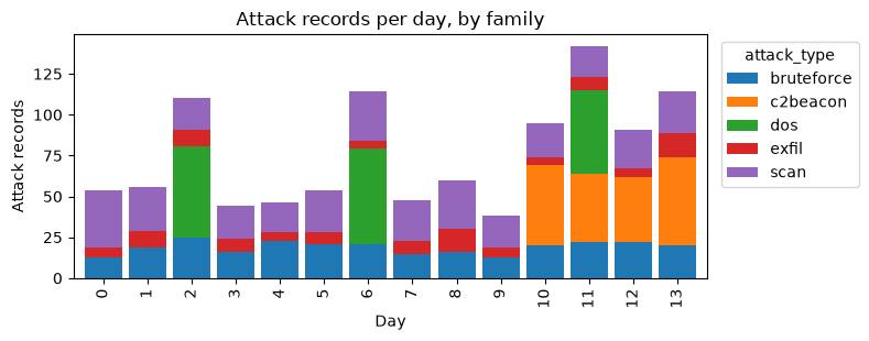
2. A detector that never raises an alert
The simplest possible detector labels every connection as normal. Its accuracy equals the share of normal records.
never_alert_accuracy = 1 - prevalence
print(f"accuracy of a detector that never alerts: {never_alert_accuracy:.4f}")
print("attacks it detects: 0")
accuracy of a detector that never alerts: 0.9719 attacks it detects: 0
3. A logistic regression trained on the past and tested on the future
We train on days 0 to 9 and test on days 10 to 13, the way a detector is used in practice, learning from the past and judged on what comes next. Unit 2 explains why this split matters. The duration, byte, packet and connection-count features (count and srv_count) are heavily skewed, so we take their logarithm before scaling them.
skewed = ["duration", "src_bytes", "dst_bytes", "packets", "count", "srv_count"]
plain = ["failed_logins", "serror_rate", "rerror_rate", "same_srv_rate", "dst_host_count", "hour"]
categorical = ["protocol", "service"]

prep = ColumnTransformer([
    ("log", make_pipeline(FunctionTransformer(np.log1p), StandardScaler()), skewed),
    ("num", StandardScaler(), plain),
    ("cat", OneHotEncoder(handle_unknown="ignore"), categorical),
])
model = make_pipeline(prep, LogisticRegression(max_iter=2000))

train = flows[flows["day"] <= 9]
test = flows[flows["day"] >= 10]
model.fit(train, train["label"])
score = model.predict_proba(test)[:, 1]
pred = (score >= 0.5).astype(int)

tn, fp, fn, tp = confusion_matrix(test["label"], pred).ravel()
print(f"test records: {len(test):,}, of which attacks: {test['label'].sum()}")
print(f"TP={tp}  FN={fn}  FP={fp}  TN={tn}")
test records: 10,834, of which attacks: 442 TP=139 FN=303 FP=8 TN=10384
From the four counts we compute the metrics of Lesson 1.2.
accuracy = (tp + tn) / (tp + tn + fp + fn)
recall = tp / (tp + fn)
fpr = fp / (fp + tn)
precision = tp / (tp + fp)
print(f"accuracy  {accuracy:.4f}")
print(f"recall    {recall:.3f}   (true positive rate)")
print(f"FPR       {fpr:.4f}  (false positive rate)")
print(f"precision {precision:.3f}")
never_alert_test = 1 - test["label"].mean()
print(f"accuracy of never alerting on the same test days: {never_alert_test:.4f}")
accuracy 0.9713 recall 0.314 (true positive rate) FPR 0.0008 (false positive rate) precision 0.946 accuracy of never alerting on the same test days: 0.9592
The accuracy is high, but the detector that never alerts is almost as accurate on the same days. Recall and precision describe what an analyst actually experiences. Most alerts are real, yet more than two attacks in three go unnoticed at the default threshold of 0.5. Lesson 2.3 shows how to choose a better threshold.
Which attacks were missed? The next cell gives recall per family.
test_types = test["attack_type"].to_numpy()
recall_by_type = {}
for t in sorted(set(test_types) - {"normal"}):
    mask = test_types == t
    recall_by_type[t] = pred[mask].mean()
    print(f"{t:<11} {mask.sum():>4} records, recall {recall_by_type[t]:.2f}")
bruteforce 84 records, recall 0.44 c2beacon 185 records, recall 0.00 dos 51 records, recall 0.76 exfil 33 records, recall 0.00 scan 89 records, recall 0.71
4. From error rates to alerts per day
The test period covers four days. Dividing the alerts by four gives the daily load on an analyst.
days = test["day"].nunique()
alerts_per_day = (tp + fp) / days
false_alerts_per_day = fp / days
print(f"alerts per day: {alerts_per_day:.1f}, of which false: {false_alerts_per_day:.1f}")
alerts per day: 36.8, of which false: 2.0
5. Precision at a lower base rate
In this dataset about 3% of records are attacks, far more than in most real networks. Precision depends on that base rate, but the true and false positive rates do not (Lesson 1.2). We can therefore ask what precision the same detector would have if only 0.1% of connections were attacks.
def precision_at(base_rate, tpr, fpr):
    return tpr * base_rate / (tpr * base_rate + fpr * (1 - base_rate))

test_base_rate = test["label"].mean()
precision_low = precision_at(0.001, recall, fpr)
print(f"base rate in the test days: {test_base_rate:.2%}, precision {precision_at(test_base_rate, recall, fpr):.3f}")
print(f"base rate of 0.1%:          precision {precision_low:.3f}")
base rate in the test days: 4.08%, precision 0.946 base rate of 0.1%: precision 0.290
The same detector, with the same error rates, would produce mostly false alerts in a network where attacks are thirty times rarer.
6. What the dataset contains
Lesson 1.3 describes the dataset column by column. The cells below count what it contains, so that every number quoted about the dataset comes from the data itself. First, the two sites. Site A is the main office and site B a smaller branch office.
by_site = flows.groupby("site").agg(records=("label", "size"), hosts=("src_host", "nunique"),
                                    attacks=("label", "sum"), base_rate=("label", "mean"))
print(by_site)
print()
print(f"days: {flows['day'].min()} to {flows['day'].max()}, from {flows['timestamp'].min()} to {flows['timestamp'].max()}")
print(f"columns: {flows.shape[1]}")
records hosts attacks base_rate site A 25512 140 504 0.019755 B 12361 60 562 0.045466 days: 0 to 13, from 2025-03-03T00:03:05Z to 2025-03-16T23:59:51Z columns: 21
Next, the cell below counts the records of each attack family and gives the first and last day on which it appears, the number of days on which it appears and the share of its records at site B.
attacks = flows[flows["label"] == 1]
family = attacks.groupby("attack_type").agg(records=("label", "size"), first_day=("day", "min"),
                                            last_day=("day", "max"), days_present=("day", "nunique"))
family["share_site_b"] = attacks.groupby("attack_type")["site"].apply(lambda s: (s == "B").mean())
print(family.round(2))
records first_day last_day days_present share_site_b attack_type bruteforce 266 0 13 14 0.61 c2beacon 185 10 13 4 0.51 dos 165 2 11 3 0.47 exfil 112 0 13 14 0.51 scan 338 0 13 14 0.51
Some records were logged twice, as happens when a collector retransmits. An exact duplicate agrees with an earlier record in every column, including the timestamp to the second.
dup = flows.duplicated(keep="first")
print(f"duplicate records: {dup.sum():,} of {len(flows):,} ({dup.mean():.1%}), of which attacks: {flows.loc[dup, 'label'].sum()}")
duplicate records: 1,103 of 37,873 (2.9%), of which attacks: 26
The column ticket_opened records whether an analyst opened a ticket after investigating the connection. It is filled in after the fact, so a detector could never use it to decide. Used as if it were a detector, it would look excellent, which is exactly why it must be excluded (Unit 2 shows the effect on a model).
ticket_rate = flows.groupby("label")["ticket_opened"].mean()
ticket_precision = flows.loc[flows["ticket_opened"] == 1, "label"].mean()
print(f"tickets opened for attacks: {ticket_rate[1]:.1%}, for normal records: {ticket_rate[0]:.1%}")
print(f"share of tickets that concern attacks: {ticket_precision:.1%}")
tickets opened for attacks: 85.8%, for normal records: 1.0% share of tickets that concern attacks: 71.2%
Several benign behaviors resemble attacks. Each can be picked out with a simple rule on the normal records: administrators who mistype a password produce failed logins; nightly backups upload large volumes at night; the IT team's authorized vulnerability scanner (host A010, on days 3 and 9) opens many connections; and a misconfigured service keeps retrying a closed port, so the far side never returns a byte.
normal = flows[flows["label"] == 0]
night = [0, 1, 2, 3, 4, 23]
is_scanner = (normal["src_host"] == "A010") & normal["day"].isin([3, 9]) & (normal["count"] >= 20)
lookalikes = {
    "failed logins (admins)": normal["failed_logins"] > 0,
    "large uploads at night (backups)": (normal["src_bytes"] > 100_000) & normal["hour"].isin(night),
    "IT vulnerability scanner": is_scanner,
    "no reply bytes (misconfigured service)": (normal["dst_bytes"] == 0) & ~is_scanner,
}
for name, mask in lookalikes.items():
    print(f"{name:<40} {mask.sum():>5} normal records")
print()
print("attack records with failed logins:", int((attacks["failed_logins"] > 0).sum()))
print("attack records with large uploads:", int((attacks["src_bytes"] > 100_000).sum()))
failed logins (admins) 432 normal records
large uploads at night (backups)           462 normal records
IT vulnerability scanner                   169 normal records
no reply bytes (misconfigured service)     232 normal records

attack records with failed logins: 235
attack records with large uploads: 112
Each look-alike resembles an attack family on the features that make that family visible, so no single threshold separates them. The next plot compares the distribution of bytes sent for normal and attack records. Backups and exfiltration share the right-hand peak.
fig, ax = plt.subplots(figsize=(8, 3))
bins = np.arange(0, 8.75, 0.25)
for lab, name in [(0, "normal"), (1, "attack")]:
    x = np.log10(flows.loc[flows["label"] == lab, "src_bytes"] + 1)
    ax.hist(x, bins=bins, density=True, histtype="step", linewidth=1.5, label=name)
ax.set_xlabel("log10(src_bytes + 1)")
ax.set_ylabel("Density within class")
ax.legend()
plt.tight_layout()
plt.show()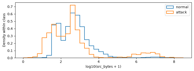
Try this:
- Count the attack records per family at each site. Which family is most concentrated at site B?
- Remove the duplicates with
flows.drop_duplicates()and recompute the base rate. Predict first whether it moves up or down. - Find a feature on which the c2beacon records look different from normal web traffic. (A good place to start is
dst_host_countand the spread ofsrc_bytes.)
Results summary
These are the numbers quoted in the lesson text.
results = {
    "n_records": int(len(flows)),
    "n_attacks": int(flows["label"].sum()),
    "prevalence": float(prevalence),
    "never_alert_accuracy": float(never_alert_accuracy),
    "never_alert_accuracy_test": float(never_alert_test),
    "n_test": int(len(test)),
    "n_test_attacks": int(test["label"].sum()),
    "test_base_rate": float(test_base_rate),
    "tp": int(tp), "fn": int(fn), "fp": int(fp), "tn": int(tn),
    "accuracy": float(accuracy),
    "recall": float(recall),
    "fpr": float(fpr),
    "precision": float(precision),
    "recall_c2beacon": float(recall_by_type["c2beacon"]),
    "alerts_per_day": float(alerts_per_day),
    "false_alerts_per_day": float(false_alerts_per_day),
    "precision_at_0_1pct": float(precision_low),
    "n_columns": int(flows.shape[1]),
    "n_days": int(flows["day"].nunique()),
    "first_timestamp": str(flows["timestamp"].min()),
    "last_timestamp": str(flows["timestamp"].max()),
    "n_normal": int((flows["label"] == 0).sum()),
    "n_unique_records": int(len(flows) - dup.sum()),
    "n_duplicates": int(dup.sum()),
    "duplicate_share": float(dup.mean()),
    "n_duplicate_attacks": int(flows.loc[dup, "label"].sum()),
    "ticket_rate_attack": float(ticket_rate[1]),
    "ticket_rate_normal": float(ticket_rate[0]),
    "ticket_precision": float(ticket_precision),
    "n_admin_failed_logins": int(lookalikes["failed logins (admins)"].sum()),
    "n_backups": int(lookalikes["large uploads at night (backups)"].sum()),
    "n_scanner": int(lookalikes["IT vulnerability scanner"].sum()),
    "n_misconfig": int(lookalikes["no reply bytes (misconfigured service)"].sum()),
    "n_attack_failed_logins": int((attacks["failed_logins"] > 0).sum()),
    "n_attack_large_uploads": int((attacks["src_bytes"] > 100_000).sum()),
}
for s in ["A", "B"]:
    results[f"n_records_site_{s.lower()}"] = int(by_site.loc[s, "records"])
    results[f"n_hosts_site_{s.lower()}"] = int(by_site.loc[s, "hosts"])
    results[f"n_attacks_site_{s.lower()}"] = int(by_site.loc[s, "attacks"])
    results[f"base_rate_site_{s.lower()}"] = float(by_site.loc[s, "base_rate"])
# Numbers used in the Unit 1 exercises: the base rate without duplicates, and the expected
# daily alerts of this detector at a site with 100,000 connections a day and a base rate of 0.1%.
dedup = flows.drop_duplicates()
results["n_attacks_dedup"] = int(dedup["label"].sum())
results["prevalence_dedup"] = float(dedup["label"].mean())
results["false_alerts_100k_0_1pct"] = float(100_000 * (1 - 0.001) * fpr)
results["true_alerts_100k_0_1pct"] = float(100_000 * 0.001 * recall)
results["alerts_100k_0_1pct"] = results["false_alerts_100k_0_1pct"] + results["true_alerts_100k_0_1pct"]
dos_days = sorted(int(d) for d in attacks.loc[attacks["attack_type"] == "dos", "day"].unique())
results["dos_days"] = ", ".join(str(d) for d in dos_days[:-1]) + f" and {dos_days[-1]}"
for t, row in family.iterrows():
    results[f"n_{t}"] = int(row["records"])
    results[f"first_day_{t}"] = int(row["first_day"])
    results[f"days_present_{t}"] = int(row["days_present"])
    results[f"share_site_b_{t}"] = float(row["share_site_b"])
for k, v in results.items():
    print(f"{k:<24} {v}")

# Data for the figures of Lesson 1.3: attack records per day by family, and histograms of two features.
export = {"days": [int(d) for d in range(int(flows["day"].max()) + 1)],
          "per_day": {t: [int(v) for v in per_day.reindex(range(int(flows["day"].max()) + 1), fill_value=0)[t]]
                      for t in per_day.columns}}
hist_specs = {"log_src_bytes": (np.log10(flows["src_bytes"] + 1), np.arange(0, 8.75, 0.25)),
              "count": (flows["count"], np.arange(0, 205, 5))}
for name, (values, edges) in hist_specs.items():
    export[name] = {"edges": [float(e) for e in edges]}
    for lab, cls in [(0, "normal"), (1, "attack")]:
        counts, _ = np.histogram(values[flows["label"] == lab], bins=edges)
        export[name][cls] = [int(c) for c in counts]

# When the course build runs this notebook, it saves the numbers for the lesson pages.
if os.environ.get("COURSE_RESULTS"):
    import json
    with open(os.environ["COURSE_RESULTS"], "w") as f:
        json.dump({"results": results, "data": export}, f)
n_records 37873 n_attacks 1066 prevalence 0.028146700815884666 never_alert_accuracy 0.9718532991841153 never_alert_accuracy_test 0.9592025106147314 n_test 10834 n_test_attacks 442 test_base_rate 0.0407974893852686 tp 139 fn 303 fp 8 tn 10384 accuracy 0.9712940742108178 recall 0.31447963800904977 fpr 0.0007698229407236335 precision 0.9455782312925171 recall_c2beacon 0.0 alerts_per_day 36.75 false_alerts_per_day 2.0 precision_at_0_1pct 0.2902354694198377 n_columns 21 n_days 14 first_timestamp 2025-03-03T00:03:05Z last_timestamp 2025-03-16T23:59:51Z n_normal 36807 n_unique_records 36770 n_duplicates 1103 duplicate_share 0.029123650093734323 n_duplicate_attacks 26 ticket_rate_attack 0.8583489681050657 ticket_rate_normal 0.010079604423071698 ticket_precision 0.7115085536547434 n_admin_failed_logins 432 n_backups 462 n_scanner 169 n_misconfig 232 n_attack_failed_logins 235 n_attack_large_uploads 112 n_records_site_a 25512 n_hosts_site_a 140 n_attacks_site_a 504 base_rate_site_a 0.01975540921919097 n_records_site_b 12361 n_hosts_site_b 60 n_attacks_site_b 562 base_rate_site_b 0.04546557721867163 n_attacks_dedup 1040 prevalence_dedup 0.028283927114495514 false_alerts_100k_0_1pct 76.905311778291 true_alerts_100k_0_1pct 31.447963800904976 alerts_100k_0_1pct 108.35327557919597 dos_days 2, 6 and 11 n_bruteforce 266 first_day_bruteforce 0 days_present_bruteforce 14 share_site_b_bruteforce 0.6127819548872181 n_c2beacon 185 first_day_c2beacon 10 days_present_c2beacon 4 share_site_b_c2beacon 0.5081081081081081 n_dos 165 first_day_dos 2 days_present_dos 3 share_site_b_dos 0.4666666666666667 n_exfil 112 first_day_exfil 0 days_present_exfil 14 share_site_b_exfil 0.5089285714285714 n_scan 338 first_day_scan 0 days_present_scan 14 share_site_b_scan 0.5059171597633136