Unit 1 · Lesson 1.1
Where machine learning helps in security
Security teams were filtering mail, scanning files and inspecting network traffic long before machine learning became fashionable, and most of that work was done with rules written by people. Learned models now sit beside those rules in mail gateways, endpoint products, fraud systems and analysis tools. This lesson explains what it means for a program to learn from data, surveys where learning is used in security and what it adds to rules, sets out the properties that make security a harder setting for machine learning than most, and introduces the second subject of the course, the security of machine learning systems themselves. It ends with a map of the course.
What learning from data means
Mitchell (1997) gives a definition that fits security problems well. A computer program learns from experience \(E\) with respect to a class of tasks \(T\) and a performance measure \(P\) if its performance at tasks in \(T\), as measured by \(P\), improves with experience \(E\). For a mail filter, the task is to decide whether an incoming message is junk, the experience is a collection of messages that users have already sorted, and the performance measure might be the share of junk caught at a fixed rate of legitimate mail wrongly discarded. Naming all three before writing any code forces the questions that decide whether a project succeeds. A filter evaluated on overall accuracy and one evaluated on how much legitimate mail it loses are different products, even if they share a model.
Most of this course works with supervised learning. Each example is a pair \((x, y)\), where \(x\) is a vector of features describing an event (the bytes of a connection, the words of a message, the imports of an executable) and \(y \in \{0, 1\}\) is its label, 1 for an attack and 0 for normal. A model \(f_\theta\) with parameters \(\theta\) maps features to a score \(s = f_\theta(x)\), and the detector raises an alert when the score reaches a threshold \(t\). Training chooses \(\theta\) to make a loss \(\ell\), which measures how wrong a score is for a given label, small on average over the \(n\) training examples,
The quantity \(\hat{R}\) is the empirical risk. What we actually care about is the average loss on the events the detector will meet after deployment, the expected risk
where \(\mathcal{P}_{\text{deploy}}\) is the distribution of events in deployment. The usual justification for minimizing \eqref{eq:empirical-risk} as a way to make \eqref{eq:expected-risk} small assumes that the training examples are drawn from the same distribution as the deployment events. Mitchell notes that most theory of machine learning rests on this assumption, and that it must often be violated in practice. In security it is violated as a matter of routine, because attackers change their behavior, networks change their software, and some of the attacks that matter most are new ones that are not yet in the training data. Much of this course is about the consequences.
Unsupervised learning drops the labels and looks for structure in \(x\) alone, such as clusters of similar hosts or events that are unusual relative to the rest. Unit 4 applies it to anomaly detection.
Where learning is used
Table 1.1 lists the main application areas with an example from the literature for each. The examples are chosen because they show the shape of the problem clearly, and the list is far from complete.
| Area | Event \(x\) (label \(y\)) | Example |
|---|---|---|
| Spam filtering | e-mail message (junk or legitimate) | naive Bayes filter (Sahami et al., 1998) |
| Phishing and malicious URLs | URL and its host data (malicious or benign) | linear classifiers on URL features (Ma et al., 2009) |
| Malware detection | executable file (malicious or benign) | boosted trees on byte n-grams (Kolter and Maloof, 2006) |
| Network intrusion detection | connection or flow (attack or normal) | anomaly detectors, as critiqued by Sommer and Paxson (2010) |
| Fraud detection | transaction or account (fraudulent or not) | supervised and unsupervised scoring (Bolton and Hand, 2002) |
| User and entity behavior | a user's activity on one day (insider threat or not) | recurrent network scoring log activity (Tuor et al., 2017) |
| Vulnerability discovery | code fragment (vulnerable or not) | recurrent network on code slices (Li et al., 2018) |
| Threat intelligence from text | sentence of a report (describes attack behavior or not) | language model classifier (Satvat et al., 2021) |
Table 1.1. Application areas of machine learning in security. Each row names the event that is classified, with its label in parentheses, and one published study as an example.
In spam filtering, Sahami et al. (1998) trained a naive Bayes classifier on the words of e-mail messages together with hand-chosen features such as particular phrases and the domain type of the sender. Because discarding a legitimate message costs far more than letting one junk message through, they labeled a message as junk only if its estimated probability of being junk exceeded 99.9%, an early application of the cost reasoning of Lesson 1.2. Ma et al. (2009) classified URLs as malicious or benign from lexical features of the URL and properties of its host, training on benign URLs from two web directories and malicious URLs from a phishing blocklist and a spam feed. In malware detection, Kolter and Maloof (2006) represented 1,971 benign and 1,651 malicious executables by byte sequences and found that boosted decision trees separated them best, with an area under the receiver operating characteristic (ROC) curve of 0.996 (Unit 2 explains this measure).
In network intrusion detection, Sommer and Paxson (2010) observed that operational deployments relied almost exclusively on signature systems, despite years of research on learned anomaly detectors; their analysis of why recurs below. For fraud, Bolton and Hand (2002) review supervised methods, which need labeled examples of fraud and can only find kinds of fraud that have occurred before, and unsupervised methods, which flag the accounts most dissimilar from the norm. User and entity behavior analytics applies the same idea to the activity of employees and machines. Tuor et al. (2017) trained deep and recurrent networks, without labels, on per-user daily counts of logon, web, e-mail, file and removable-device activity from a synthetic insider-threat dataset, and ranked user-days by anomaly score so that analysts with a fixed daily budget could review the most anomalous first.
Two further areas apply learning to code and text. Li et al. (2018) built VulDeePecker, which splits programs into small, semantically related slices of code and trains a recurrent network to flag vulnerable ones. Chakraborty et al. (2022) later found that the performance of several deep learning vulnerability detectors dropped by more than 50% in a realistic setting. They traced the drop to problems in the training data, such as duplication and an unrealistic share of vulnerable code, and to models that learned artifacts such as particular variable and function names instead of the causes of vulnerabilities. Threat intelligence arrives largely as prose in reports and blogs, and Satvat et al. (2021) used a BERT classifier, among other language-processing steps, to separate sentences that describe attack behavior from the rest before extracting the behavior as a graph.
Show the answer
\(T\) is ranking user-days by how likely they are to involve insider-threat activity. \(E\) is a history of activity logs, mostly from benign users. A suitable \(P\) is the recall of insider-threat cases among the top \(k\) ranked user-days, where \(k\) is the number analysts can review; Tuor et al. (2017) summarize recall over a range of daily budgets. Accuracy would be poor because threat events are a tiny share of all user-days, so a model that ranks no one as suspicious would be almost perfectly accurate (Lesson 1.2).
Signatures and learned detectors
A signature or rule is a precise description of something known to be malicious, written by an analyst. Snort, an open-source network intrusion detection system, matches packets against rules that combine addresses, ports, flags and byte patterns in the payload. Its author describes writing a rule for a new exploit by running the exploit on a test network, finding a byte sequence unique to it, and condensing that into a rule, which takes only minutes once the signature is known (Roesch, 1999). Blocklists of known malicious URLs or file hashes are signatures in the same sense.
Signatures have two strengths. They are precise, so a well-written rule rarely fires on benign traffic, and their alerts explain themselves, because the rule that matched says what was seen. Their weakness is the converse of their precision. A signature matches what someone has already described, so it misses new attacks and new variants until a rule is written, and the rule set needs constant maintenance. Sahami et al. (1998) made this argument against hand-built mail filters, and Ma et al. (2009) note that many malicious sites are missing from blocklists because they are too new, were never evaluated, or were evaluated incorrectly.
A learned detector generalizes from examples, so it can flag variants that resemble known attacks without anyone writing a rule for them. Sommer and Paxson (2010) argue that machine learning is much better at finding activity similar to what it has seen than at discovering genuinely novel attacks. A classifier needs examples of the attacks it is meant to find, and a detector trained on normal traffic alone would need a close-to-perfect model of normality to single out the few events that matter. Generalization comes with more false positives and weaker explanations, since a learned score is harder to interpret than a matched rule. Figure 1.1 illustrates the two failure modes in two dimensions.
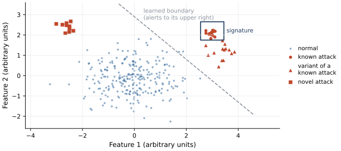
Figure 1.1. An illustration with synthetic points in two arbitrary feature dimensions (not data from the course). The signature, the small square, matches all 18 known attacks and nothing else. The learned boundary, the dashed line, also catches all 14 variants of the known attack and raises alerts on 2 of the 260 normal points. Neither detects the 10 novel attacks at the upper left, which resemble nothing in the training data.
The two kinds of detector fail on different events, which is the argument for running them together. Suppose a detector raises an alert on an event with probability \(p_{\mathrm{s}}\) from the signatures and \(p_{\mathrm{l}}\) from the learned model, and the two fire independently given the type of event. An alert from either one then occurs with probability
Equation \eqref{eq:union} applies to attacks and to normal events alike, so combining detectors adds their detections and also their false alarms.
As a worked example, take a network with 1,000,000 normal events a day, 50 instances of known attacks and 50 instances of new variants. The signatures detect known attacks with probability 0.98, variants with probability 0.10, and fire on normal events with probability \(2 \times 10^{-6}\). The learned detector detects known attacks with probability 0.90, variants with probability 0.60, and fires on normal events with probability \(10^{-4}\). The signatures alone find \(49 + 5 = 54\) attacks a day, a recall (share of attacks detected) of 0.54, with 2 false alerts and a precision (share of alerts that are real attacks) of 0.96. Lesson 1.2 defines both measures formally. The learned detector alone finds \(45 + 30 = 75\) attacks, a recall of 0.75, with 100 false alerts and a precision of 0.43. Together, by \eqref{eq:union}, they detect known attacks with probability \(1 - 0.02 \times 0.10 = 0.998\) and variants with probability \(1 - 0.90 \times 0.40 = 0.64\), so they find \(49.9 + 32 = 81.9\) attacks a day, a recall of 0.82, at the cost of about 102 false alerts and a precision of 0.45. The learned component adds most of the coverage of variants and almost all of the false alerts. Whether the trade is worth making depends on the alert budget, a question Unit 2 answers quantitatively. The independence assumption is optimistic, because events that evade one detector often evade the other for the same reason.
What makes security different
Machine learning succeeds in many domains with the same algorithms that struggle in security. Sommer and Paxson (2010) attribute the difference to properties of the security setting, and Arp et al. (2022) later showed how often the resulting pitfalls appear in published work. In their study of 30 papers from the four leading security conferences, sampling bias (data that do not represent the true distribution of the security problem) and data snooping (training with information that would not be available in practice) were at least partly present in 90% and 73% of the papers respectively, and every paper suffered from at least three of the ten pitfalls they define. Six properties of the setting underlie many of these problems.
The first is an adversary. Attackers adjust their activity to avoid detection, so defenders and attackers improve in response to each other. Sommer and Paxson (2010) call evasion a fundamentally hard problem for any intrusion detector, while also arguing that sophisticated attacks on the learning algorithm itself require effort that many untargeted attackers will not spend, so the threat model should say which attackers matter. Biggio and Roli (2018) trace attacks on learned spam filters back to 2004.
The second is concept drift, change over time in the relationship between features and labels or in the distribution of events. Arp et al. (2022) note that data distributions in security are often non-stationary because of new attacks and new technologies, and that ignoring time when splitting data is a common form of data snooping. Pendlebury et al. (2019) examined Android malware classifiers with published F1 scores (a summary of precision and recall defined in Lesson 1.2) of up to 0.99 and found that they performed far worse once training data came strictly before test data and the test set held a realistic share of malware.
The third is extreme class imbalance. Attacks are rare among the events a detector inspects, which makes accuracy uninformative and pushes precision down unless the false positive rate (the share of normal events that raise an alert) is very small. Lesson 1.2 derives this, following Axelsson (2000). Arp et al. (2022) list among their pitfalls the base-rate fallacy, which is judging a detector without regard to how rare attacks are (the base rate).
The fourth is the cost of errors. A false positive consumes analyst time, and a false negative can leave a compromised system in place. Sommer and Paxson (2010) contrast this with product recommendation and character recognition, where errors are cheap or easily corrected.
The fifth is the lack of labels and ground truth. Labeled attack data is scarce, sensitive and often wrong. Sommer and Paxson (2010) describe the shortage of public datasets, caused largely by the privacy of network traffic, and Arp et al. (2022) observe that for network attacks and malware reliable labels are typically not available, so researchers fall back on heuristics and external services. Lesson 1.3 shows what this has done to public benchmark datasets.
The sixth is the semantic gap, the distance between what a model reports and what an operator needs to act on. A report that a host's traffic "did not match the normal profile" leaves the analyst to work out what happened, and Sommer and Paxson (2010) argue that understanding which operationally relevant activity a system can and cannot detect matters more than tuning its parameters.
Show the answer
Class imbalance makes the accuracy hard to interpret, because if attacks are rare a detector that never alerts is also highly accurate; recall, the false positive rate and precision at a realistic base rate are needed. Concept drift makes the shuffled split hard to interpret, because records from later days, including later attack variants, are in the training set, so the test measures performance on a past the model has already seen rather than on the future it will face (Arp et al. call this temporal snooping). The lack of reliable labels could also be named if the labels were produced by a heuristic.
The security of machine learning itself
The second half of the course reverses the point of view. Once a model makes security decisions, or any decisions that someone has an interest in changing, the model becomes a target. Figure 1.2 shows where learned components sit in a detection pipeline and where attacks on them enter.
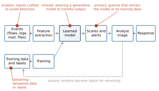
Figure 1.2. A detection pipeline with a learned model, and the points where four classes of attack on machine learning enter (red markers). Evasion manipulates the events the model scores. Poisoning tampers with the training data or its labels, including the analyst verdicts that are fed back for retraining (dashed path). Privacy attacks use the model's outputs to extract the model or information about its training data. Misuse, a class specific to generative models, steers a model into producing output its operator meant to prevent. The attack classes follow NIST AI 100-2e2025 (Vassilev et al., 2025).
Biggio and Roli (2018) organize these attacks by the attacker's goal and capability. The goal may be an integrity violation, evading detection without disrupting normal operation; an availability violation, degrading the system for legitimate users; or a privacy violation, obtaining information about the system, its users or its data. The capability determines when the attacker acts, at training time by poisoning the data or at test time by manipulating inputs. The taxonomy published by NIST in March 2025, NIST AI 100-2e2025 (Vassilev et al., 2025), uses the same three objectives for predictive models and groups the attacks into evasion, poisoning and privacy. For generative models it adds a fourth objective, misuse enablement, in which the attacker circumvents restrictions placed on a model's outputs. In the same study of 30 papers, Arp et al. (2022) found an inappropriate threat model, one that ignores attacks on the learning system, at least partly present in more than half of the papers.
These attacks follow from the properties described earlier. Poisoning exploits the lack of trustworthy labels, evasion exploits the adversary, and retraining on fresh data to counter drift opens a door for poisoning. Units 7 to 10 study them in turn.
Show the answer
The attacker can generate activity that resembles their real attack but is harmless, so that analysts investigate it, judge it benign, and label it normal. After retraining, the model treats that kind of activity as normal, and the real attack passes. This is poisoning, because it acts on the training data through its labels. The same feedback loop shows why retraining needs controls on where labels come from.
A map of the course
The course has twelve units in five parts. Units 1 to 4 build the foundations: the measures and pitfalls of this unit, data preparation and evaluation without leakage (Unit 2), supervised classifiers applied to intrusion and phishing detection (Unit 3), and clustering and anomaly detection (Unit 4). Units 5 and 6 cover deep learning, from backpropagation and autoencoders to convolutional and sequence models, together with reinforcement learning. Units 7 and 8 attack and defend machine learning: threat models and evasion, then poisoning, privacy attacks, adversarial training and differential privacy. Units 9 to 11 turn to generative models and governance: synthetic media and its detection, the security of language models and agents, and risk frameworks, fairness and documentation. Unit 12 is a capstone project in which you plan, run and report a study of your own using the evaluation checklist built up over the course.
Lab 1
A first look at the network data
Open in ColabRead with outputsNotebook on GitHubAbout 1 minute to run on a laptop CPU
Lab 1 loads the course dataset and trains a first detector on it. It is the companion to all three lessons of this unit, and Lesson 1.3 describes the dataset in detail.
Summary
A program learns when its performance at a task, by a stated measure, improves with experience, and most of this course works with supervised classifiers that score events and raise an alert when the score reaches a threshold. Learning is used for spam, phishing, malware, intrusions, fraud, insider threats, vulnerable code and threat reports. It complements signatures, which are precise but miss what nobody has described, by generalizing to variants at the cost of more false alerts and less transparent decisions. Adversaries, drift, rare attacks, costly errors, scarce labels and the semantic gap make the security setting harder than most, and the models themselves can be evaded, poisoned, probed for private information and misused, which is the subject of the second half of the course.
References
- Arp, D., Quiring, E., Pendlebury, F., Warnecke, A., Pierazzi, F., Wressnegger, C., Cavallaro, L., and Rieck, K. (2022). Dos and don'ts of machine learning in computer security. Proceedings of the 31st USENIX Security Symposium, 3971-3988. https://www.usenix.org/conference/usenixsecurity22/presentation/arp
- Axelsson, S. (2000). The base-rate fallacy and the difficulty of intrusion detection. ACM Transactions on Information and System Security, 3(3), 186-205. https://doi.org/10.1145/357830.357849
- Biggio, B., and Roli, F. (2018). Wild patterns: Ten years after the rise of adversarial machine learning. Pattern Recognition, 84, 317-331. https://doi.org/10.1016/j.patcog.2018.07.023
- Bolton, R. J., and Hand, D. J. (2002). Statistical fraud detection: A review. Statistical Science, 17(3), 235-255. https://doi.org/10.1214/ss/1042727940
- Chakraborty, S., Krishna, R., Ding, Y., and Ray, B. (2022). Deep learning based vulnerability detection: Are we there yet?. IEEE Transactions on Software Engineering, 48(9), 3280-3296. https://doi.org/10.1109/TSE.2021.3087402
- Kolter, J. Z., and Maloof, M. A. (2006). Learning to detect and classify malicious executables in the wild. Journal of Machine Learning Research, 7, 2721-2744. https://www.jmlr.org/papers/v7/kolter06a.html
- Li, Z., Zou, D., Xu, S., Ou, X., Jin, H., Wang, S., Deng, Z., and Zhong, Y. (2018). VulDeePecker: A deep learning-based system for vulnerability detection. Proceedings of the 2018 Network and Distributed System Security Symposium (NDSS). https://doi.org/10.14722/ndss.2018.23158
- Ma, J., Saul, L. K., Savage, S., and Voelker, G. M. (2009). Beyond blacklists: Learning to detect malicious web sites from suspicious URLs. Proceedings of the 15th ACM SIGKDD International Conference on Knowledge Discovery and Data Mining, 1245-1254. https://doi.org/10.1145/1557019.1557153
- Mitchell, T. M. (1997). Machine learning. McGraw-Hill.
- Pendlebury, F., Pierazzi, F., Jordaney, R., Kinder, J., and Cavallaro, L. (2019). TESSERACT: Eliminating experimental bias in malware classification across space and time. Proceedings of the 28th USENIX Security Symposium, 729-746. https://www.usenix.org/conference/usenixsecurity19/presentation/pendlebury
- Roesch, M. (1999). Snort: Lightweight intrusion detection for networks. Proceedings of LISA '99, the 13th Systems Administration Conference, 229-238. https://www.usenix.org/legacy/event/lisa99/full_papers/roesch/roesch.pdf
- Sahami, M., Dumais, S., Heckerman, D., and Horvitz, E. (1998). A Bayesian approach to filtering junk e-mail. Learning for Text Categorization: Papers from the 1998 Workshop, AAAI Technical Report WS-98-05, 55-62. https://cdn.aaai.org/Workshops/1998/WS-98-05/WS98-05-009.pdf
- Satvat, K., Gjomemo, R., and Venkatakrishnan, V. N. (2021). Extractor: Extracting attack behavior from threat reports. 2021 IEEE European Symposium on Security and Privacy (EuroS&P), 598-615. https://doi.org/10.1109/EuroSP51992.2021.00046
- Sommer, R., and Paxson, V. (2010). Outside the closed world: On using machine learning for network intrusion detection. 2010 IEEE Symposium on Security and Privacy, 305-316. https://doi.org/10.1109/SP.2010.25
- Tuor, A., Kaplan, S., Hutchinson, B., Nichols, N., and Robinson, S. (2017). Deep learning for unsupervised insider threat detection in structured cybersecurity data streams. The AAAI Workshop on Artificial Intelligence for Cyber Security (WS-17-04), 224-231. Association for the Advancement of Artificial Intelligence. Also available as arXiv:1710.00811. https://arxiv.org/abs/1710.00811
- Vassilev, A., Oprea, A., Fordyce, A., Anderson, H., Davies, X., and Hamin, M. (2025). Adversarial machine learning: A taxonomy and terminology of attacks and mitigations. National Institute of Standards and Technology. NIST AI 100-2e2025, March 2025. https://doi.org/10.6028/NIST.AI.100-2e2025