Unit 11 · Lesson 11.3
Model cards, datasheets and audits
Governing a detector requires that people other than its builders understand it. The people who decide whether to deploy it, the analysts who act on its alerts, the people whose accounts it locks and the auditors who check it later all need to know what it was built for, what data shaped it, how it was evaluated and where it fails. This lesson presents two documentation formats that have become standard, model cards for trained models and datasheets for datasets, and an internal audit process that uses them. It then lists what an audit of a security model should check, and shows how to monitor a deployed detector so that the documentation stays true.
Model cards
Mitchell et al. (2019) proposed that every released model be accompanied by a short document, a model card, that reports its performance across the conditions and groups relevant to its use. Their template has nine sections. Model details give the developer, date, version, model type and training algorithm. Intended use states the primary uses and users and the uses that are out of scope. Factors name the groups, instruments and environments across which performance may vary. Metrics say which measures are reported and why, at which decision threshold, and how uncertainty is estimated. Evaluation data and training data describe the datasets and their preprocessing. Quantitative analyses report the metrics separately for each factor and for combinations of factors. Ethical considerations and caveats and recommendations close the card.
The central idea is disaggregated evaluation. A single aggregate metric hides the conditions under which a model fails, so the card reports results per factor. For a security detector, the factors that matter are rarely demographic categories alone. They include the site or business unit (Lab 11), the attack family (in Lab 1, and again in Lab 11, the detector missed every command-and-control beaconing record and every exfiltration record on the test days), the time period (Unit 2), the operating system or device type, and the language of the text for detectors that read messages. The metrics are the ones this course has used throughout, reported at the deployed operating point: true positive rate, false positive rate, precision at the deployment base rate, and alerts per day against the alert budget, each with an interval.
A model card is also where intended use is fixed in writing. A detector evaluated for ranking alerts for analyst review has not been evaluated for blocking traffic automatically, and its card should say so. Writing it down makes it visible when the detector is later used for something that was never tested.
Show the answer
Useful additions include the following. The base rate of phishing in the evaluation set, with precision and false positive rate at the deployed threshold instead of accuracy, since accuracy is dominated by the benign class (Lesson 1.2). Whether the evaluation emails come from a period after the training emails and were deduplicated against them (Unit 2). Results per factor, such as language, sender type, attachment versus link lures, and new campaigns versus known ones. Intervals on every rate. A statement of intended use (quarantine with review, or deletion) and of known failure modes, including how the classifier behaves on emails crafted to evade it (Unit 7).
Datasheets for datasets
A model inherits the properties of its data, and much of what goes wrong in security machine learning goes wrong there: labels produced by the very signatures the model is supposed to improve on, duplicates that leak between training and test sets, attack traffic generated in a lab that looks nothing like the attacks in a real network, time stamps that place the test set before the training set. Gebru et al. (2021) proposed that every dataset be accompanied by a datasheet answering a standard set of questions, organized in seven sections: motivation; composition; collection process; preprocessing, cleaning and labeling; uses; distribution; and maintenance.
For a security dataset, several of their questions carry particular weight. Under composition, they ask whether the data contain confidential information and whether instances are related (records that belong to the same connection or host break the independence that a random split assumes). Under collection process, they ask over what time frame the data were collected and by what mechanism, which determines whether a temporal evaluation is possible at all. Under preprocessing, cleaning and labeling, they ask what labeling was done, which for a security dataset means who or what produced the labels; a dataset labeled by an intrusion detection system rewards models that imitate that system. Under uses, they ask what the dataset should not be used for. The course dataset is documented in this spirit in Lesson 1.3 and in the generator's own description, which states that it is synthetic, that benign traffic includes behavior resembling attacks, that one family appears only in the last days, that some records are logged twice, and that the column ticket_opened is filled in after investigation and must never be used as a feature.
Audits
An audit checks whether a system and the claims made about it hold up. Raji et al. (2020) proposed an internal audit framework, SMACTR, with five stages. Scoping clarifies the audit's objective by reviewing the system's intended use and the principles it must meet. Mapping reviews what is already in place, identifies the internal stakeholders and collaborators, and begins a failure modes and effects analysis that ranks risks for later testing. Artifact collection gathers the documentation of the development process, including model cards and datasheets. Testing executes tests that gauge whether the system complies with the values and requirements prioritized during scoping. Reflection compares the results with the expectations set during scoping and records the remaining risks and the actions to address them. Figure 11.6 lays out the stages with the artifacts each produces for a security detector.
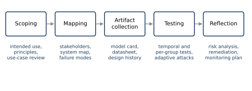
Figure 11.6. The five stages of the SMACTR internal audit framework of Raji et al. (2020), with examples of the artifacts each stage produces when the system under audit is a security detector. Arrows show the order of the stages.
For a security model, the testing stage should cover at least the points in the table below, each of which is developed in an earlier lesson or in this one.
| Check | What the auditor looks for | Course reference |
|---|---|---|
| Data provenance | Where training and test data came from, who labeled them and how, known artifacts, duplicates, legal basis for any personal data | Lessons 1.3 and 2.1 |
| Evaluation protocol | Split in time or by group, no leakage of identifiers or post-incident fields, threshold chosen without the test set | Lesson 2.2; Lab 2 |
| Base rate and alert budget | Precision and alerts per day at the deployment base rate, not only at the test-set rate | Lesson 1.2; Lesson 2.3 |
| Disaggregated performance | Rates per site, group, attack family and period, with intervals | Lesson 11.2; Lab 11 |
| Calibration | Whether scores mean the same thing across groups and over time | Lesson 2.3; Lab 11 |
| Robustness | Behavior under evasion, poisoning and, for language-model components, injection, with adaptive attacks | Units 7, 8 and 10 |
| Drift monitoring | Which rates are tracked after deployment, with what limits, and who is alerted | This lesson |
| Incident response | Who can change the threshold, retrain or roll back, and how affected people are informed | Lesson 11.1 (Govern and Manage) |
Figure 11.7 shows one of these checks from Lab 11. At both sites most points lie above the diagonal, so the detector's scores understate the risk, and site B's points lie further above it. The gap matters most in the lowest score bin, which holds almost all connections. Attacks that the detector misses receive low scores, and because attacks make up a larger share of site B's connections, the missed ones make up a larger share of its lowest bin.
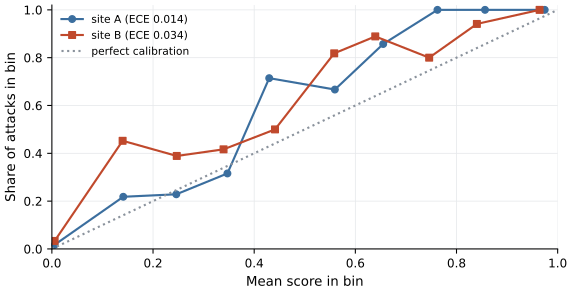
Figure 11.7. Calibration of the Lab 11 detector on the test days, per site. Each point is one of ten equal-width score bins; its horizontal position is the mean score in the bin and its vertical position the share of attacks among the bin's connections. The dotted line marks perfect calibration. The expected calibration error (ECE) in the legend averages the absolute vertical distance to the line, weighted by the number of connections in each bin; most connections fall in the lowest bin.
In Lab 11 the expected calibration error was 0.014 at site A and 0.034 at site B. A downstream rule that converts scores into actions with a single cost threshold (Lesson 1.2) would treat site B's connections as less risky than they are and act on them less often than their true risk warrants.
Monitoring after deployment
Documentation describes a system at one moment. Traffic, attackers and the organization change, so an audit plan specifies what is measured after deployment. Rates that can be computed without labels, such as the alert rate per site, are available immediately; rates that need labels, such as the false positive rate, become available as analysts close alerts. A simple and transparent monitor treats each week's count as a binomial sample. If the false positive rate at a site was \(p_0\) when the detector was approved and the site produces \(n\) normal connections in a week, the observed rate \(\hat{p}\) should stay below the upper control limit
in most weeks if nothing has changed. With \(p_0 = 0.002\) and \(n = 7{,}000\), the standard deviation is \(0.000534\) and the limit is \(0.0036\), so a week with 14 false alerts is typical and a week with more than 25 calls for a review. The same construction applies to the true positive rate on attacks confirmed by investigation, with \(p_0\) the approved true positive rate, \(n\) the number of attacks confirmed in the week, and the lower limit \(p_0 - 3\sqrt{p_0(1-p_0)/n}\) in place of the upper one, because a fall in that rate is what signals a problem. It applies likewise to each site or group separately, which is how the gap measured in an audit is kept from widening unnoticed.
Show the answer
Per-site thresholds that equalized the false positive rate on the training days stopped equalizing it on the test days, because the benign traffic that determined the thresholds changed. The authorized vulnerability scanner ran at site A on two training days and produced 131 of the 180 false alerts at site A's threshold in that period, so site A's threshold was set high. The scanner did not run during the test days, and site A's false positive rate fell well below site B's. A false positive rate depends only on the scores of normal connections, so the new attack family of the test days played no part in this. Any equalized quantity is a property of thresholds and data together, so when the data distribution shifts, the property has to be measured again. Monitoring per-group rates with limits such as equation \eqref{eq:ucl} turns that into a routine check.
What the lab shows
Lab 11
Auditing a detector across two sites
Open in ColabRead with outputsNotebook on GitHubAbout 1 minute to run on a laptop CPU
The last part of Lab 11 assembles a model card for its detector, with its results filled in from the variables the lab computes: model details, intended use (ranking for analyst review at a target false positive rate, not automated blocking), factors (site and attack family), metrics with bootstrap intervals, evaluation data with per-site base rates, a table of per-site results, recall per attack family, the false alerts each site bore, and caveats that include the families the detector missed and the failure of thresholds equalized in advance. Because the card's measured values and its target false positive rate are read from the lab's variables, rerunning the lab updates them; descriptive settings typed into the card, such as the feature description and the split days, have to be edited by hand if they change.
Summary
Model cards report what a model is for, how it was evaluated and how its performance varies across the factors that matter, at the operating point where it is used and with uncertainty stated. Datasheets record where data came from, how it was labeled and what it must not be used for, which in security covers most of the pitfalls of the earlier units. An internal audit such as SMACTR scopes, maps, collects these artifacts, tests the system against its claims and reflects on what remains. For a security model the tests cover provenance, evaluation protocol, base rate and alert budget, disaggregated performance, calibration, robustness, drift monitoring and incident response. Because the data and the attackers change, the audit ends with a monitoring plan, such as binomial control limits on per-group error rates, that keeps the documentation true after deployment.
References
- Gebru, T., Morgenstern, J., Vecchione, B., Vaughan, J. W., Wallach, H., Daumé III, H., and Crawford, K. (2021). Datasheets for datasets. Communications of the ACM, 64(12), 86-92. https://doi.org/10.1145/3458723
- Mitchell, M., Wu, S., Zaldivar, A., Barnes, P., Vasserman, L., Hutchinson, B., Spitzer, E., Raji, I. D., and Gebru, T. (2019). Model cards for model reporting. Proceedings of the Conference on Fairness, Accountability, and Transparency, 220-229. https://doi.org/10.1145/3287560.3287596
- Raji, I. D., Smart, A., White, R. N., Mitchell, M., Gebru, T., Hutchinson, B., Smith-Loud, J., Theron, D., and Barnes, P. (2020). Closing the AI accountability gap: Defining an end-to-end framework for internal algorithmic auditing. Proceedings of the 2020 Conference on Fairness, Accountability, and Transparency, 33-44. https://doi.org/10.1145/3351095.3372873