Unit 11 · Lab 11
Auditing a detector across two sites
Lab 11
Auditing a detector across two sites
Open in ColabRead with outputsNotebook on GitHubAbout 1 minute to run on a laptop CPU
# On Google Colab, install the scikit-learn version the course was built with.
# On your own computer, install requirements.txt instead; this cell then does nothing.
import subprocess, sys
if "google.colab" in sys.modules:
    subprocess.run([sys.executable, "-m", "pip", "install", "-q", "scikit-learn==1.9.0"], check=True)
Lab 11. Auditing a detector across two sites
The course dataset comes from two office sites, site A (the main office) and site B (the branch office). Site B has a higher share of attacks than site A and runs more remote administration. A detector that treats every connection in the same way can still distribute its errors unevenly between the sites, and the people behind those connections (whose accounts are locked or whose machines are reimaged after an alert) bear the cost. This lab audits a detector in the way Lesson 11.3 describes and produces a short model card from the results. It runs in under a minute.
You will:
- train a detector on days 0 to 9 and test it on days 10 to 13, choosing its threshold from out-of-fold scores on the training days;
- measure, for each site, the base rate, the true positive rate, false positive rate, precision and alert rate with bootstrap 95% intervals, and the calibration of the scores;
- see how one global threshold distributes errors between the sites;
- compute per-site thresholds that equalize the false positive rate, then the true positive rate, and measure what each choice costs;
- check whether thresholds equalized on past data stay equalized on new data;
- write a model card in Markdown from the numbers computed here.
The site is used only to group the results. It is not a feature of the detector, and neither is the source host. The data is synthetic (Lesson 1.3); the sites stand in for any two groups of people or systems that a security decision affects.
import os

import numpy as np
import pandas as pd
import matplotlib.pyplot as plt
from IPython.display import Markdown, display

from sklearn.compose import ColumnTransformer
from sklearn.linear_model import LogisticRegression
from sklearn.metrics import roc_curve
from sklearn.model_selection import GroupKFold, cross_val_predict
from sklearn.pipeline import make_pipeline
from sklearn.preprocessing import FunctionTransformer, OneHotEncoder, StandardScaler

LOCAL = "../../data/flows.csv"
URL = "https://raw.githubusercontent.com/aalbata/machine-learning-for-cybersecurity/main/data/flows.csv"
flows = pd.read_csv(LOCAL if os.path.exists(LOCAL) else URL)

skewed = ["duration", "src_bytes", "dst_bytes", "packets", "count", "srv_count"]
plain = ["failed_logins", "serror_rate", "rerror_rate", "same_srv_rate", "dst_host_count", "hour"]
categorical = ["protocol", "service"]
# Never used as features: label, attack_type, ticket_opened (filled in after investigation),
# site and src_host (the grouping variable and an identifier), timestamp and day.

train = flows[flows["day"] <= 9]
test = flows[flows["day"] >= 10]
print(f"train days 0-9: {len(train):,} records, {train['label'].sum()} attacks")
print(f"test days 10-13: {len(test):,} records, {test['label'].sum()} attacks")
train days 0-9: 27,039 records, 624 attacks test days 10-13: 10,834 records, 442 attacks
1. Base rates differ between the sites
Before looking at any model, the audit records how common attacks are at each site in each period. Every later comparison has to be read against these numbers.
base_table = flows.assign(period=np.where(flows["day"] <= 9, "train", "test")).groupby(["period", "site"])["label"].agg(
    records="size", attacks="sum", base_rate="mean")
print(base_table.round(4))
base_rate_test = {s: float(test.loc[test["site"] == s, "label"].mean()) for s in "AB"}
n_test = {s: int((test["site"] == s).sum()) for s in "AB"}
n_test_attacks = {s: int(test.loc[test["site"] == s, "label"].sum()) for s in "AB"}
records attacks base_rate
period site
test A 7212 209 0.0290
B 3622 233 0.0643
train A 18300 295 0.0161
B 8739 329 0.0376
2. Train the detector and choose a threshold without touching the test days
The detector is the logistic regression of Lab 1, with the same features and preprocessing. To choose a threshold we need scores on data the model was not fitted to. Out-of-fold scores provide them. The ten training days are split into five folds of whole days, each fold is scored by a model trained on the other four (Lesson 2.2), and the threshold is read from these scores. The folds are not ordered in time, so some training days are scored by models fitted on later days. This is less strict than the time-ordered validation that Lesson 2.2 recommends for choosing a threshold, but the test days, which follow all ten training days, never influence the choice. The final model is then refitted on all ten days and applied to the test days.
def make_model():
    prep = ColumnTransformer([
        ("log", make_pipeline(FunctionTransformer(np.log1p), StandardScaler()), skewed),
        ("num", StandardScaler(), plain),
        ("cat", OneHotEncoder(handle_unknown="ignore"), categorical),
    ])
    return make_pipeline(prep, LogisticRegression(max_iter=2000))

s_cal = cross_val_predict(make_model(), train, train["label"], groups=train["day"], cv=GroupKFold(5),
                          method="predict_proba")[:, 1]
model = make_model().fit(train, train["label"])
s_test = model.predict_proba(test)[:, 1]
y_cal, y_test = train["label"].to_numpy(), test["label"].to_numpy()
g_cal, g_test = train["site"].to_numpy(), test["site"].to_numpy()
3. One global threshold
The team can investigate about one false alert per 100 normal connections, so the global threshold is set to give an overall false positive rate of 1% on the out-of-fold scores. It is then frozen and applied to the test days.
TARGET_FPR = 0.01

def threshold_for_fpr(scores, y, fpr):
    """Smallest threshold whose false positive rate on (scores, y) does not exceed fpr."""
    neg = np.sort(scores[y == 0])[::-1]
    k = int(np.floor(fpr * len(neg)))
    return float(neg[k]) + 1e-12

def threshold_for_tpr(scores, y, tpr):
    """Largest threshold whose true positive rate on (scores, y) is at least tpr."""
    pos = np.sort(scores[y == 1])[::-1]
    k = int(np.ceil(tpr * len(pos))) - 1
    return float(pos[max(k, 0)])

t_global = threshold_for_fpr(s_cal, y_cal, TARGET_FPR)
print(f"global threshold: {t_global:.4f}")

def rates(y, alert):
    tp = int(((alert == 1) & (y == 1)).sum()); fp = int(((alert == 1) & (y == 0)).sum())
    fn = int(((alert == 0) & (y == 1)).sum()); tn = int(((alert == 0) & (y == 0)).sum())
    return {"tpr": tp / (tp + fn) if tp + fn else np.nan,
            "fpr": fp / (fp + tn) if fp + tn else np.nan,
            "precision": tp / (tp + fp) if tp + fp else np.nan,
            "alert_rate": (tp + fp) / len(y), "tp": tp, "fp": fp, "fn": fn, "tn": tn}

def bootstrap(y, alert, reps=1000, seed=0):
    """Percentile 95% intervals from resampling connections within one site."""
    r = np.random.default_rng(seed)
    n = len(y)
    out = {k: [] for k in ("tpr", "fpr", "precision", "alert_rate")}
    for _ in range(reps):
        i = r.integers(0, n, n)
        m = rates(y[i], alert[i])
        for k in out:
            out[k].append(m[k])
    return {k: (float(np.nanpercentile(v, 2.5)), float(np.nanpercentile(v, 97.5))) for k, v in out.items()}

def audit(thresholds, label):
    rows = []
    for s in "AB":
        m = g_test == s
        alert = (s_test[m] >= thresholds[s]).astype(int)
        r = rates(y_test[m], alert)
        ci = bootstrap(y_test[m], alert, seed=ord(s))
        rows.append({"policy": label, "site": s, "threshold": thresholds[s], **r,
                     **{f"{k}_lo": ci[k][0] for k in ci}, **{f"{k}_hi": ci[k][1] for k in ci}})
    return pd.DataFrame(rows)

cols = ["site", "threshold", "tp", "fp", "tpr", "tpr_lo", "tpr_hi", "fpr", "fpr_lo", "fpr_hi", "precision", "alert_rate"]
global_audit = audit({"A": t_global, "B": t_global}, "global")
print(global_audit[cols].round(4).to_string(index=False))
global threshold: 0.2427 site threshold tp fp tpr tpr_lo tpr_hi fpr fpr_lo fpr_hi precision alert_rate A 0.2427 72 33 0.3445 0.2772 0.4112 0.0047 0.0031 0.0065 0.6857 0.0146 B 0.2427 94 23 0.4034 0.3360 0.4667 0.0068 0.0041 0.0098 0.8034 0.0323
Both sites face the same threshold. The cell above prints, for each site, the counts of true and false alerts, the two error rates with their bootstrap intervals, precision and the share of connections that raise an alert. Read the false positive rates first, since they say how often a person at each site is disturbed for nothing. The rate at site B is higher than at site A, and so is its true positive rate. The false positive rates, however, rest on a few dozen false alerts and the true positive rates on about two hundred attacks at each site, and both pairs of intervals overlap. An audit reports the rates, the counts behind them and the intervals together. The alert rates also differ, partly because site B has more attacks; equal alert rates (demographic parity) would require the detector to alert on site B's connections no more often than on site A's despite that difference.
The overall false positive rate on the test days is also only about half of the 1% chosen on the training days. Section 6 explains why.
Which attack families drive the true positive rate? The next cell breaks recall down by family and site.
alert_global = (s_test >= t_global).astype(int)
fam = test.assign(alert=alert_global)
fam = fam[fam["label"] == 1].groupby(["attack_type", "site"])["alert"].agg(["size", "mean"]).unstack("site")
print(fam.round(3))
size mean site A B A B attack_type bruteforce 31 53 0.548 0.585 c2beacon 91 94 0.000 0.000 dos 27 24 0.852 0.875 exfil 19 14 0.000 0.000 scan 41 48 0.780 0.875
Command-and-control beaconing (c2beacon) first appears on day 10, and the detector catches none of it at either site. Exfiltration (exfil) also occurs on the training days, yet the detector misses all of it on the test days as well. A per-family table like this belongs in every audit, because an aggregate recall hides which threats the detector cannot see at all.
4. Calibration within each site
A score is calibrated within a group when, among that group's connections that receive a score near \(p\), about a fraction \(p\) are attacks. The next cell bins the test scores into ten equal-width bins and compares the mean score with the observed share of attacks in each bin, per site. The expected calibration error (ECE) averages the absolute gap over bins, weighted by the number of connections in each bin.
def reliability(scores, y, bins=10):
    edges = np.linspace(0, 1, bins + 1)
    idx = np.clip(np.digitize(scores, edges) - 1, 0, bins - 1)
    mean_s, frac, count = [], [], []
    for b in range(bins):
        m = idx == b
        if m.sum() == 0:
            continue
        mean_s.append(float(scores[m].mean())); frac.append(float(y[m].mean())); count.append(int(m.sum()))
    mean_s, frac, count = map(np.array, (mean_s, frac, count))
    ece = float(np.sum(count * np.abs(mean_s - frac)) / count.sum())
    return mean_s, frac, count, ece

calib = {}
fig, ax = plt.subplots(figsize=(4.5, 4))
for s, c in (("A", "#3B6E9E"), ("B", "#C0492C")):
    m = g_test == s
    ms, fr, ct, ece = reliability(s_test[m], y_test[m])
    calib[s] = {"mean_score": ms.tolist(), "fraction": fr.tolist(), "count": ct.tolist(), "ece": ece,
                "brier": float(np.mean((s_test[m] - y_test[m]) ** 2))}
    ax.plot(ms, fr, "o-", color=c, label=f"site {s} (ECE {ece:.3f})")
    print(f"site {s}: ECE {ece:.4f}, Brier score {calib[s]['brier']:.4f}")
ax.plot([0, 1], [0, 1], ":", color="gray")
ax.set_xlabel("Mean score in bin"); ax.set_ylabel("Share of attacks in bin"); ax.legend()
plt.tight_layout(); plt.show()
site A: ECE 0.0135, Brier score 0.0197 site B: ECE 0.0340, Brier score 0.0397
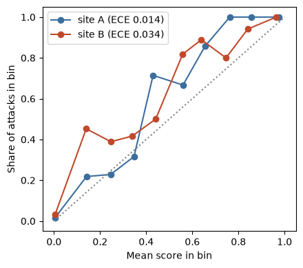
Points below the diagonal mean the scores overstate the risk; points above mean they understate it. In the test days the detector misses two families entirely, so many attacks receive low scores and the share of attacks in the lowest bin exceeds the mean score there. Attacks make up a larger share of site B's connections, so the missed ones are a larger share of its low-score bins, and in the four lowest bins (scores below 0.4) its points lie further above the diagonal than site A's. The lowest bin holds almost all connections and therefore dominates the ECE, and site B's gap there is the larger one, which is why site B has the larger ECE.
5. Per-site thresholds and what equalization would have cost
A per-site threshold is the post-processing remedy of Hardt, Price and Srebro (Lesson 11.2), which leaves the model alone and chooses a separate threshold for each group so that a chosen error rate is equal. To see the mechanism and its cost exactly, this section chooses the thresholds on the test days themselves, the way an auditor looks back on a period that is over. Section 6 asks what happens when the thresholds have to be chosen in advance.
First, equal false positive rates. Each site receives the threshold at which its own false positive rate equals the overall false positive rate of the global threshold, so the total number of false alerts stays about the same.
overall = rates(y_test, alert_global)
t_eqfpr = {s: threshold_for_fpr(s_test[g_test == s], y_test[g_test == s], overall["fpr"]) for s in "AB"}
eqfpr_audit = audit(t_eqfpr, "equal FPR")
print(f"overall test FPR at the global threshold: {overall['fpr']:.4f}")
print(eqfpr_audit[cols].round(4).to_string(index=False))
overall test FPR at the global threshold: 0.0054 site threshold tp fp tpr tpr_lo tpr_hi fpr fpr_lo fpr_hi precision alert_rate A 0.2180 75 37 0.3589 0.2921 0.4255 0.0053 0.0036 0.007 0.6696 0.0155 B 0.2813 93 18 0.3991 0.3320 0.4635 0.0053 0.0030 0.008 0.8378 0.0306
Second, equal true positive rates (equal opportunity). Each site receives the threshold at which its recall equals the overall recall of the global threshold.
t_eqtpr = {s: threshold_for_tpr(s_test[g_test == s], y_test[g_test == s], overall["tpr"]) for s in "AB"}
eqtpr_audit = audit(t_eqtpr, "equal TPR")
print(f"overall test TPR at the global threshold: {overall['tpr']:.4f}")
print(eqtpr_audit[cols].round(4).to_string(index=False))
overall test TPR at the global threshold: 0.3756 site threshold tp fp tpr tpr_lo tpr_hi fpr fpr_lo fpr_hi precision alert_rate A 0.1749 79 52 0.3780 0.312 0.4466 0.0074 0.0056 0.0094 0.6031 0.0182 B 0.3294 88 15 0.3777 0.312 0.4384 0.0044 0.0024 0.0069 0.8544 0.0284
The table below compares the three policies over the whole test period: alerts raised, attacks detected, false alerts, overall precision, and the gap between the sites (B minus A) in each error rate.
summary = []
for df in (global_audit, eqfpr_audit, eqtpr_audit):
    tp, fp = df["tp"].sum(), df["fp"].sum()
    summary.append({"policy": df["policy"].iloc[0], "alerts": int(tp + fp), "detected": int(tp), "false_alerts": int(fp),
                    "precision": tp / (tp + fp), "tpr_gap": float(df["tpr"].iloc[1] - df["tpr"].iloc[0]),
                    "fpr_gap": float(df["fpr"].iloc[1] - df["fpr"].iloc[0])})
summary = pd.DataFrame(summary)
print(summary.round(4).to_string(index=False))
policy alerts detected false_alerts precision tpr_gap fpr_gap global 222 166 56 0.7477 0.0589 0.0021 equal FPR 223 168 55 0.7534 0.0403 0.0000 equal TPR 234 167 67 0.7137 -0.0003 -0.0030
Each policy equalizes the rate it targets and leaves a gap in the other, and the two policies need different thresholds. With equal false positive rates, site B keeps the higher point estimate of the true positive rate, although the two intervals overlap widely. With equal true positive rates, the gap in false positive rates reverses, so that site A now has the higher false positive rate, and the total number of false alerts rises. With two groups whose score distributions differ, a single pair of deterministic thresholds rarely equalizes both rates at once; Hardt, Price and Srebro show that equalized odds may require randomizing between two thresholds for one group.
6. Do thresholds equalized on the past stay equal?
In deployment the thresholds must be chosen before the data arrives. The next cell equalizes the false positive rate on the out-of-fold scores of the training days, at the same 1% target, and then applies those thresholds to the test days.
t_prosp = {s: threshold_for_fpr(s_cal[g_cal == s], y_cal[g_cal == s], TARGET_FPR) for s in "AB"}
prosp_audit = audit(t_prosp, "equal FPR, chosen in advance")
cal_fpr = {s: float((s_cal[(g_cal == s) & (y_cal == 0)] >= t_prosp[s]).mean()) for s in "AB"}
print("FPR on the training days (out of fold):", {s: round(v, 4) for s, v in cal_fpr.items()})
print(prosp_audit[cols].round(4).to_string(index=False))
scan_host = (train["src_host"] == "A010").to_numpy()
fa_A = (g_cal == "A") & (y_cal == 0) & (s_cal >= t_prosp["A"])
fa_all = (y_cal == 0) & (s_cal >= t_global)
train_fa = {"A_prosp": int(fa_A.sum()), "A_prosp_scanner": int((fa_A & scan_host).sum()),
            "global": int(fa_all.sum()), "global_scanner": int((fa_all & scan_host).sum())}
print(f"site A false alerts on the training days at its own threshold: {train_fa['A_prosp']}, "
      f"from the scanner host A010: {train_fa['A_prosp_scanner']}")
print(f"false alerts on the training days at the global threshold: {train_fa['global']}, "
      f"from the scanner host A010: {train_fa['global_scanner']}")
print("days of the scanner host's false alerts:", sorted(set(train.loc[fa_all & scan_host, "day"].tolist())))
FPR on the training days (out of fold): {'A': 0.01, 'B': 0.01}
site threshold tp fp tpr tpr_lo tpr_hi fpr fpr_lo fpr_hi precision alert_rate
A 0.3116 69 14 0.3301 0.2620 0.3934 0.0020 0.0010 0.0031 0.8313 0.0115
B 0.1619 101 33 0.4335 0.3682 0.4938 0.0097 0.0068 0.0132 0.7537 0.0370
site A false alerts on the training days at its own threshold: 180, from the scanner host A010: 131
false alerts on the training days at the global threshold: 264, from the scanner host A010: 146
days of the scanner host's false alerts: [3, 9]
The thresholds equalize the false positive rate on the days they were fitted to and not on the test days, where the gap is wider than under the global threshold. The last lines of the output show why. The IT team's authorized vulnerability scanner, host A010, runs at site A on days 3 and 9 and not during the test period. On the training days it produced most of site A's false alerts at site A's own threshold, and more than half of all false alerts at the global threshold. Site A therefore looked noisier in the past than it is now, its threshold was set high, and on the test days its false positive rate fell far below the 1% target. The same traffic explains why the global threshold gives only about half of its target rate on the test days. Equalization is a property of a threshold and a data distribution together. It has to be re-measured on every new period, which is why the audit plan in Lesson 11.3 includes monitoring per-group rates after deployment.
7. A model card generated from the results
The card below follows the sections proposed by Mitchell et al. (2019), with the training data summarized under model details instead of in a section of its own. Every number in it is read from the variables computed above, so rerunning the lab rewrites the card.
def pct(x, d=1):
    return f"{100 * x:.{d}f}%"

g = global_audit.set_index("site")

def ci(site, k, d=1):
    return f"{pct(g.loc[site, k], d)} ({pct(g.loc[site, k + '_lo'], d)} to {pct(g.loc[site, k + '_hi'], d)})"

site_rows = "\n".join(f"| {s} | {ci(s, 'tpr')} | {ci(s, 'fpr', 2)} | {ci(s, 'precision')} | {ci(s, 'alert_rate')} | "
                      f"{calib[s]['ece']:.3f} |" for s in "AB")
family_names = {"bruteforce": "brute force", "c2beacon": "command-and-control beaconing", "dos": "denial of service",
                "exfil": "exfiltration", "scan": "scanning"}
family_rows = "\n".join(f"| {family_names[k]} | {int(fam.loc[k, ('size', 'A')])} | {pct(float(fam.loc[k, ('mean', 'A')]))} | "
                        f"{int(fam.loc[k, ('size', 'B')])} | {pct(float(fam.loc[k, ('mean', 'B')]))} |" for k in fam.index)
missed = [family_names[k] for k in fam.index if fam.loc[k, ("mean", "A")] == 0 and fam.loc[k, ("mean", "B")] == 0]
missed_text = " or ".join(missed) if missed else "no"
card = f"""### Model card for the connection detector (course example)

#### Model details

Logistic regression (scikit-learn `LogisticRegression`) on twelve numeric features, six of them log-transformed, and two one-hot encoded categorical features. Trained on days 0 to 9 of the synthetic course dataset `flows.csv`. Threshold {t_global:.3f}, chosen from out-of-fold scores on the training days for an overall false positive rate of {pct(TARGET_FPR)}.

#### Intended use

Ranking connection records for analyst review at a target false positive rate of {pct(TARGET_FPR)} (about one false alert per {round(1 / TARGET_FPR):,} normal connections). Not intended for automated blocking, or for any action against a person, without review by an analyst.

#### Factors

Results are reported per site (A, main office; B, branch office) and per attack family. Site and host identifiers are not model inputs.

#### Metrics

True positive rate, false positive rate, precision and alert rate at the deployed threshold, with bootstrap 95% intervals (1,000 resamples of connections within each site); expected calibration error (ECE) with ten bins.

#### Evaluation data

Days 10 to 13: {n_test['A']:,} connections at site A ({pct(base_rate_test['A'])} attacks) and {n_test['B']:,} at site B ({pct(base_rate_test['B'])} attacks). The test days include an attack family, command-and-control beaconing, that is absent from the training days.

#### Quantitative analyses

| Site | True positive rate | False positive rate | Precision | Alert rate | ECE |
|---|---|---|---|---|---|
{site_rows}

Recall per attack family on the test days:

| Family | Attacks at site A | Recall at site A | Attacks at site B | Recall at site B |
|---|---|---|---|---|
{family_rows}

#### Ethical considerations

False alerts cost analyst time and, if acted on, can lead to locked accounts and reimaged machines for the people at each site. Under the global threshold, {int(g.loc['A','fp'])} false alerts fell on site A and {int(g.loc['B','fp'])} on site B during the four test days.

#### Caveats and recommendations

Synthetic data; one split in time; intervals reflect resampling of connections, not variation between days. The detector caught none of the {missed_text} records at either site. The overall false positive rate on the test days was {pct(overall['fpr'], 2)}, below the {pct(TARGET_FPR)} target, because traffic from an authorized vulnerability scanner raised the threshold on the training days. Per-site thresholds that equalize the false positive rate on past data did not keep it equal on the test days. Monitor per-site rates weekly, re-check thresholds after any change in traffic, and do not use the detector for families it has not been tested on.
"""
display(Markdown(card))
<IPython.core.display.Markdown object>
Try this
- Lower the target false positive rate to
TARGET_FPR = 0.005and rerun. Predict whether the ratio of the false positive rates of the two sites grows or shrinks, then check. - Add
siteto the features. Does the gap in the false positive rate at a global threshold change? Would you deploy that model, and what would you have to document? - Replace connection-level resampling in
bootstrapwith resampling of whole days (four test days). How wide do the intervals become, and what does that say about evidence from four days?
Results summary
results = {
    "n_test_A": n_test["A"], "n_test_B": n_test["B"],
    "n_test_attacks_A": n_test_attacks["A"], "n_test_attacks_B": n_test_attacks["B"],
    "base_rate_test_A": base_rate_test["A"], "base_rate_test_B": base_rate_test["B"],
    "target_fpr": TARGET_FPR, "t_global": t_global,
    "overall_tpr": overall["tpr"], "overall_fpr": overall["fpr"],
    "t_eqfpr_A": t_eqfpr["A"], "t_eqfpr_B": t_eqfpr["B"], "t_eqtpr_A": t_eqtpr["A"], "t_eqtpr_B": t_eqtpr["B"],
    "t_prosp_A": t_prosp["A"], "t_prosp_B": t_prosp["B"],
    "cal_fpr_A": cal_fpr["A"], "cal_fpr_B": cal_fpr["B"],
    "ece_A": calib["A"]["ece"], "ece_B": calib["B"]["ece"],
    "brier_A": calib["A"]["brier"], "brier_B": calib["B"]["brier"],
    "recall_c2beacon_A": float(fam.loc["c2beacon", ("mean", "A")]),
    "recall_c2beacon_B": float(fam.loc["c2beacon", ("mean", "B")]),
    "recall_exfil_A": float(fam.loc["exfil", ("mean", "A")]),
    "recall_exfil_B": float(fam.loc["exfil", ("mean", "B")]),
    "train_fa_A_prosp": train_fa["A_prosp"], "train_fa_A_prosp_scanner": train_fa["A_prosp_scanner"],
    "train_fa_global": train_fa["global"], "train_fa_global_scanner": train_fa["global_scanner"],
}
for df, tag in ((global_audit, "global"), (eqfpr_audit, "eqfpr"), (eqtpr_audit, "eqtpr"), (prosp_audit, "prosp")):
    for _, row in df.iterrows():
        for k in ("tpr", "fpr", "precision", "alert_rate", "tpr_lo", "tpr_hi", "fpr_lo", "fpr_hi",
                  "precision_lo", "precision_hi", "alert_rate_lo", "alert_rate_hi"):
            results[f"{tag}_{k}_{row['site']}"] = float(row[k])
        results[f"{tag}_tp_{row['site']}"] = int(row["tp"])
        results[f"{tag}_fp_{row['site']}"] = int(row["fp"])
for _, row in summary.iterrows():
    tag = {"global": "global", "equal FPR": "eqfpr", "equal TPR": "eqtpr"}[row["policy"]]
    results[f"{tag}_total_alerts"] = int(row["alerts"])
    results[f"{tag}_total_detected"] = int(row["detected"])
    results[f"{tag}_total_false_alerts"] = int(row["false_alerts"])
    results[f"{tag}_total_precision"] = float(row["precision"])
    results[f"{tag}_tpr_gap"] = float(row["tpr_gap"])
    results[f"{tag}_fpr_gap"] = float(row["fpr_gap"])
results["fpr_ratio_global"] = float(global_audit["fpr"].iloc[1] / global_audit["fpr"].iloc[0])
results["alert_rate_ratio_global"] = float(global_audit["alert_rate"].iloc[1] / global_audit["alert_rate"].iloc[0])

export = {"calibration": calib, "roc": {}, "policies": {}}
for s in "AB":
    m = g_test == s
    f_, t_, _ = roc_curve(y_test[m], s_test[m])
    keep = np.unique(np.linspace(0, len(f_) - 1, 400).astype(int))
    export["roc"][s] = {"fpr": f_[keep].tolist(), "tpr": t_[keep].tolist()}
for df in (global_audit, eqfpr_audit, eqtpr_audit, prosp_audit):
    export["policies"][df["policy"].iloc[0]] = df[["site", "threshold", "tpr", "fpr", "precision", "alert_rate",
                                                   "tpr_lo", "tpr_hi", "fpr_lo", "fpr_hi"]].to_dict("records")
for k, v in results.items():
    print(f"{k:<32} {v}")

# When the course build runs this notebook, it saves the numbers for the lesson pages.
if os.environ.get("COURSE_RESULTS"):
    import json
    with open(os.environ["COURSE_RESULTS"], "w") as f:
        json.dump({"results": results, "data": export}, f)
n_test_A 7212 n_test_B 3622 n_test_attacks_A 209 n_test_attacks_B 233 base_rate_test_A 0.028979478646699943 base_rate_test_B 0.06432909994478189 target_fpr 0.01 t_global 0.24268084124060385 overall_tpr 0.3755656108597285 overall_fpr 0.005388760585065435 t_eqfpr_A 0.2180438387598801 t_eqfpr_B 0.2813277205338907 t_eqtpr_A 0.17492421241870446 t_eqtpr_B 0.3293590846976326 t_prosp_A 0.31162196004162046 t_prosp_B 0.1618804737868058 cal_fpr_A 0.009997222993612885 cal_fpr_B 0.009988109393579072 ece_A 0.013518265200089353 ece_B 0.03395475362146276 brier_A 0.01970695903893347 brier_B 0.03972906704145978 recall_c2beacon_A 0.0 recall_c2beacon_B 0.0 recall_exfil_A 0.0 recall_exfil_B 0.0 train_fa_A_prosp 180 train_fa_A_prosp_scanner 131 train_fa_global 264 train_fa_global_scanner 146 global_tpr_A 0.3444976076555024 global_fpr_A 0.004712266171640726 global_precision_A 0.6857142857142857 global_alert_rate_A 0.014559068219633943 global_tpr_lo_A 0.2772094720992837 global_tpr_hi_A 0.4112210377725857 global_fpr_lo_A 0.003139258209112745 global_fpr_hi_A 0.006452057532444893 global_precision_lo_A 0.5940309296416367 global_precision_hi_A 0.7727368220015278 global_alert_rate_lo_A 0.011785912368275097 global_alert_rate_hi_A 0.01747088186356073 global_tp_A 72 global_fp_A 33 global_tpr_B 0.4034334763948498 global_fpr_B 0.0067866627323694305 global_precision_B 0.8034188034188035 global_alert_rate_B 0.032302595251242405 global_tpr_lo_B 0.33597155963302755 global_tpr_hi_B 0.4666898148148148 global_fpr_lo_B 0.00411522633744856 global_fpr_hi_B 0.009807053839211606 global_precision_lo_B 0.7289719626168224 global_precision_hi_B 0.875 global_alert_rate_lo_B 0.027056874654886803 global_alert_rate_hi_B 0.038107399226946434 global_tp_B 94 global_fp_B 23 eqfpr_tpr_A 0.3588516746411483 eqfpr_fpr_A 0.005283449950021419 eqfpr_precision_A 0.6696428571428571 eqfpr_alert_rate_A 0.01552967276760954 eqfpr_tpr_lo_A 0.29207811267852446 eqfpr_tpr_hi_A 0.42553464266230223 eqfpr_fpr_lo_A 0.003586505648915979 eqfpr_fpr_hi_A 0.007002025589458725 eqfpr_precision_lo_A 0.5794392523364486 eqfpr_precision_hi_A 0.7565339292970337 eqfpr_alert_rate_lo_A 0.012756516916250694 eqfpr_alert_rate_hi_A 0.01844148641153633 eqfpr_tp_A 75 eqfpr_fp_A 37 eqfpr_tpr_B 0.39914163090128757 eqfpr_fpr_B 0.005311301268810859 eqfpr_precision_B 0.8378378378378378 eqfpr_alert_rate_B 0.030646051905024847 eqfpr_tpr_lo_B 0.3319983193277311 eqfpr_tpr_hi_B 0.4635427048796859 eqfpr_fpr_lo_B 0.002963841138114997 eqfpr_fpr_hi_B 0.008023774145616641 eqfpr_precision_lo_B 0.7666176470588236 eqfpr_precision_hi_B 0.9042782465150404 eqfpr_alert_rate_lo_B 0.02567642186637217 eqfpr_alert_rate_hi_B 0.03645085588072887 eqfpr_tp_B 93 eqfpr_fp_B 18 eqtpr_tpr_A 0.37799043062200954 eqtpr_fpr_A 0.007425389118949022 eqtpr_precision_A 0.6030534351145038 eqtpr_alert_rate_A 0.018164170826400445 eqtpr_tpr_lo_A 0.31196369636963694 eqtpr_tpr_hi_A 0.44661200841125676 eqtpr_fpr_lo_A 0.005564254660148589 eqtpr_fpr_hi_A 0.009423220390249655 eqtpr_precision_lo_A 0.5196850393700787 eqtpr_precision_hi_A 0.6846259842519685 eqtpr_alert_rate_lo_A 0.015252357182473655 eqtpr_alert_rate_hi_A 0.021353300055463115 eqtpr_tp_A 79 eqtpr_fp_A 52 eqtpr_tpr_B 0.3776824034334764 eqtpr_fpr_B 0.004426084390675715 eqtpr_precision_B 0.8543689320388349 eqtpr_alert_rate_B 0.028437327443401435 eqtpr_tpr_lo_B 0.31196483180428136 eqtpr_tpr_hi_B 0.4383621725546743 eqtpr_fpr_lo_B 0.0023612228633541734 eqtpr_fpr_hi_B 0.006856645947966022 eqtpr_precision_lo_B 0.7818181818181819 eqtpr_precision_hi_B 0.9174335571739336 eqtpr_alert_rate_lo_B 0.023467697404748758 eqtpr_alert_rate_hi_B 0.033966040861402536 eqtpr_tp_B 88 eqtpr_fp_B 15 prosp_tpr_A 0.33014354066985646 prosp_fpr_A 0.001999143224332429 prosp_precision_A 0.8313253012048193 prosp_alert_rate_A 0.011508596783139213 prosp_tpr_lo_A 0.26199697682230433 prosp_tpr_hi_A 0.3933649289099526 prosp_fpr_lo_A 0.0009989938724422958 prosp_fpr_hi_A 0.003134863297490911 prosp_precision_lo_A 0.7472495894909688 prosp_precision_hi_A 0.9114017125837677 prosp_alert_rate_lo_A 0.009151414309484194 prosp_alert_rate_hi_A 0.014143094841930116 prosp_tp_A 69 prosp_fp_A 14 prosp_tpr_B 0.4334763948497854 prosp_fpr_B 0.009737385659486574 prosp_precision_B 0.753731343283582 prosp_alert_rate_B 0.03699613473219216 prosp_tpr_lo_B 0.3681958158995816 prosp_tpr_hi_B 0.4937729945173856 prosp_fpr_lo_B 0.006790570022693647 prosp_fpr_hi_B 0.013244061372305257 prosp_precision_lo_B 0.6772021033596649 prosp_precision_hi_B 0.8227028808134061 prosp_alert_rate_lo_B 0.03147432357813363 prosp_alert_rate_hi_B 0.04334621755935947 prosp_tp_B 101 prosp_fp_B 33 global_total_alerts 222 global_total_detected 166 global_total_false_alerts 56 global_total_precision 0.7477477477477478 global_tpr_gap 0.058935868739347363 global_fpr_gap 0.002074396560728705 eqfpr_total_alerts 223 eqfpr_total_detected 168 eqfpr_total_false_alerts 55 eqfpr_total_precision 0.7533632286995515 eqfpr_tpr_gap 0.04028995626013926 eqfpr_fpr_gap 2.7851318789439902e-05 eqtpr_total_alerts 234 eqtpr_total_detected 167 eqtpr_total_false_alerts 67 eqtpr_total_precision 0.7136752136752137 eqtpr_tpr_gap -0.00030802718853312205 eqtpr_fpr_gap -0.0029993047282733066 fpr_ratio_global 1.4402120943873673 alert_rate_ratio_global 2.218726828113907