Unit 9 · Lesson 9.1
How synthetic media is made
Synthetic media is image, video or audio content produced or altered by machine learning so that it appears to show something that did not happen. For a security team, it matters as an instrument of fraud and social engineering, a cloned voice on a telephone call or a fabricated executive on a video call, and as a source of disinformation. Detecting it and responding to it (Lessons 9.2 and 9.3) starts with knowing how it is made, because every detector exploits some trace of a particular generation process. This lesson describes the main families of generators, namely face swapping with autoencoders, generative adversarial networks, diffusion models, face reenactment and voice cloning, and what each requires of an attacker.
A taxonomy of face manipulation
The word deepfake comes from a Reddit user named "deepfakes" who, in late 2017, claimed to have developed a machine learning algorithm for swapping celebrity faces into videos (Tolosana et al., 2020). Tolosana et al. survey facial manipulation in four groups. Entire face synthesis creates faces of people who do not exist. Identity swap replaces the face of a person in a video by another person's face, which is what "deepfake" originally meant. Attribute manipulation changes properties such as age, hair or glasses. Expression swap, also called reenactment, keeps the target's identity and changes the target's facial expression and mouth movement to match a source actor. The methods differ, and so do the traces they leave.
Face swapping with a shared encoder
The original deepfake method is built from autoencoders, not from a generative adversarial network. FaceForensics++, the benchmark of Rössler et al. (2019), describes it as two autoencoders with a shared encoder, trained to reconstruct face images of the source person and of the target person respectively. Write \(E\) for the shared encoder and \(D_A\), \(D_B\) for the decoders of persons A and B. Training minimizes the reconstruction error of each person's faces through that person's decoder, written here as a squared error,
where \(\mathcal{X}_A\) and \(\mathcal{X}_B\) are aligned face crops of the two people. The encoder is shared so that it represents pose, expression and lighting in a way common to both faces, while each decoder learns to render one identity. To swap, a face of B is passed through the encoder and then through the decoder of A, \(\hat x = D_A(E(x_B))\), which renders A with B's pose and expression. The output is blended back into B's frame. In FaceForensics++, a face detector crops and aligns the faces, and the generated face is merged into the target frame with Poisson image editing. Figure 9.1 shows the arrangement.
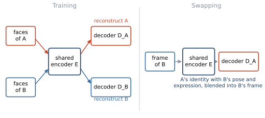
Figure 9.1. The face-swapping autoencoder of equation \eqref{eq:faceswap}. During training (left), aligned face crops of person A pass through the shared encoder \(E\) and A's decoder \(D_A\), and crops of person B through \(E\) and \(D_B\); each path is trained to reconstruct its input. To produce a swap (right), a frame of B is encoded with \(E\) and decoded with \(D_A\), so A's identity is rendered with B's pose and expression, and the result is blended into B's frame.
The method needs many images of both people and a separate model for each pair. Rössler et al. note that it has to be trained for each pair of videos, which is time-consuming, whereas graphics-based face swapping can run in real time. Public datasets were made with several implementations and refinements of this method. Li et al. list, for example, one generated with an open-source tool called faceswap-GAN, and built their own Celeb-DF dataset with an improved synthesis algorithm that raises the resolution of the synthesized faces and reduces color mismatch, inaccurate face masks and temporal flickering (Li et al., 2020).
Generative adversarial networks
A generative adversarial network (GAN) (Goodfellow et al., 2014) trains two networks against each other. The generator \(G\) maps a random vector \(z\) drawn from a simple distribution \(p_z\) to a sample \(G(z)\), and the discriminator \(D\) outputs the probability that its input came from the training data, whose distribution is \(p_{\mathrm{data}}\), rather than from \(G\). They play the minimax game
For a fixed generator whose samples have density \(p_g\), the best discriminator is
and Goodfellow et al. showed that the game's global optimum is reached when \(p_g = p_{\mathrm{data}}\), where \(D^* = 1/2\) everywhere. As a numerical check, at a point where the data density is 0.3 and the generator density is 0.1, the optimal discriminator outputs \(0.3/0.4 = 0.75\); if the generator moves density toward that point until its own density there also reaches 0.3, the output falls to \(0.3/0.6 = 0.5\). In practice the generator is trained to maximize \(\log D(G(z))\) instead of minimizing \(\log(1 - D(G(z)))\), which gives stronger gradients early in training. Figure 9.2 shows the training loop.
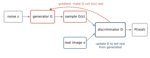
Figure 9.2. Training a generative adversarial network, equation \eqref{eq:gan}. The generator turns random noise \(z\) into a sample; the discriminator receives real training images and generated samples and outputs the probability that its input is real. The discriminator is updated to classify better, and the generator is updated through the discriminator's gradient to make its samples classified as real. The two updates alternate.
In the 2020 survey of Tolosana et al., entire face synthesis is usually performed with GANs (Tolosana et al., 2020). StyleGAN (Karras et al., 2019) generates high-resolution faces from a style-based generator, introduced the Flickr-Faces-HQ (FFHQ) dataset of face photographs, and was released with its source code and pretrained networks. Synthesized faces of this kind have been implicated in fraudulent social media profiles (Carlini and Farid, 2020). A GAN generator, like most image generators, starts from a small spatial representation and enlarges it through upsampling layers, either transposed convolutions or interpolation followed by convolution. That step matters for detection. Odena et al. (2016) showed that a transposed convolution whose kernel size is not divisible by its stride produces uneven overlap and a checkerboard pattern, and that resizing followed by convolution avoids it in the image. Lab 9 simulates exactly this step.
Diffusion models
Denoising diffusion probabilistic models (Ho et al., 2020) generate by learning to reverse a gradual noising process. The forward process adds Gaussian noise to a data point \(x_0\) over \(T\) steps according to a variance schedule \(\beta_1, \dots, \beta_T\),
where \(\mathcal{N}(x; \mu, \Sigma)\) is the Gaussian density with mean \(\mu\) and covariance \(\Sigma\), and \(I\) is the identity matrix. With \(\alpha_t = 1 - \beta_t\) and \(\bar\alpha_t = \prod_{s=1}^{t} \alpha_s\), the noisy version at any step can be drawn directly,
The reverse step \(p_\theta(x_{t-1} \mid x_t)\) is a Gaussian with mean \(\mu_\theta(x_t, t)\) and covariance \(\Sigma_\theta(x_t, t)\), learned by a network with parameters \(\theta\). Ho et al. fix the covariance \(\Sigma_\theta(x_t, t) = \sigma_t^2 I\) to untrained constants, parameterize the mean through a network \(\epsilon_\theta\) that predicts the noise added to \(x_0\), and train it with the simplified objective
where \(\epsilon \sim \mathcal{N}(0, I)\) and \(t\) is drawn uniformly. Generation starts from pure noise \(x_T\) and applies the learned reverse step \(T\) times. Ho et al. used \(T = 1000\) and a schedule rising linearly from \(\beta_1 = 10^{-4}\) to \(\beta_T = 0.02\). With that schedule, the signal coefficient \(\sqrt{\bar\alpha_t}\) in \eqref{eq:closed-form} is about 0.95 at \(t = 100\), 0.28 at \(t = 500\) and 0.0064 at \(t = 1000\), so by the last step essentially nothing of the image remains. Figure 9.3 plots both coefficients.
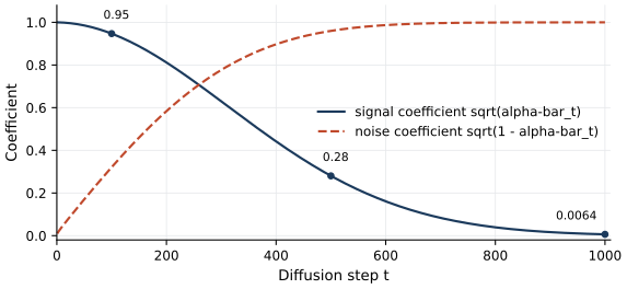
Figure 9.3. The forward process of a diffusion model with the linear schedule of Ho et al. (\(T = 1000\), \(\beta_t\) rising from \(10^{-4}\) to 0.02), computed from equation \eqref{eq:closed-form}. The signal coefficient \(\sqrt{\bar\alpha_t}\) multiplies the clean image and the noise coefficient \(\sqrt{1 - \bar\alpha_t}\) multiplies the Gaussian noise. The marked points are the values quoted in the text at \(t = 100\), 500 and 1000. Generation runs this process backward with a learned denoiser.
Running a diffusion model in pixel space is expensive. Latent diffusion (Rombach et al., 2022) trains the diffusion model in the latent space of a pretrained autoencoder, which reduces the cost while keeping image quality, and conditions the denoising network on text or other inputs through cross-attention layers, which Rombach et al. used for text-to-image synthesis among other tasks. A latent diffusion model ends with the autoencoder's decoder, which upsamples the latent representation to a full image; Lesson 9.3 describes a watermark that is built into that decoder.
Show the answer
From equation \eqref{eq:closed-form}, \(x_t = \sqrt{\bar\alpha_t}\, x_0 + \sqrt{1 - \bar\alpha_t}\, \epsilon\), so for independent \(x_0\) and \(\epsilon\) with unit variance, the variance is \(\bar\alpha_t + (1 - \bar\alpha_t) = 1\) and the noise contributes \(1 - \bar\alpha_t\). With \(\sqrt{\bar\alpha_{250}} \approx 0.72\), \(\bar\alpha_{250} \approx 0.52\), so about 48% of the variance is noise. The factor \(\sqrt{1 - \beta_t}\) in \eqref{eq:forward} keeps the total variance at 1 for any schedule, and the schedule sets how fast the share of signal decays.
Face reenactment
Reenactment changes what a target person appears to do while keeping who they are. Face2Face (Thies et al., 2016) reconstructs a three-dimensional face model of the target from a monocular video, tracks the expressions of a source actor captured live with a webcam, transfers the expression to the target model, and re-renders the target's face, retrieving a matching mouth interior from the target video. It runs in real time on commodity hardware. NeuralTextures, one of the four FaceForensics++ methods, learns a neural texture of the target together with a rendering network, trained with a photometric reconstruction loss and an adversarial loss (Rössler et al., 2019). In the FaceForensics++ user study, reenactment methods such as Face2Face and NeuralTextures were particularly hard for people to detect, because they change only expressions and leave subtle artifacts. Real-time reenactment is the capability that a live video call with a fabricated participant requires.
Voice cloning and text-to-speech
Voice cloning synthesizes speech in a particular person's voice. Jia et al. (2018) built a text-to-speech (TTS) system from three separately trained parts. The first is a speaker encoder trained on a speaker verification task (deciding whether a recording comes from a claimed speaker), which maps a few seconds of reference speech to a fixed-length embedding of the speaker's voice. The second is a sequence-to-sequence network based on Tacotron 2, which produces a spectrogram (the energy of the speech in each frequency band over time) from text conditioned on that embedding, and the third is a WaveNet-based vocoder that converts the spectrogram to a waveform. Because the speaker encoder generalizes, the system can speak in the voice of people unseen during training, from a short untranscribed sample and without retraining. The authors noted the potential for misuse, such as impersonating someone's voice without consent. For an attacker, the implication is that a short recording of a person, from a public talk, a voicemail greeting or a social media video, can be enough material to start from.
Show the answer
First, the original identity-swap deepfakes are made with autoencoders that share an encoder, not with GANs. Reenactment methods such as Face2Face are based on three-dimensional face models and rendering, and newer content may come from diffusion models. Second, even within a family, a detector trained on the traces of one generator often fails on another (Lesson 9.2). The video's generation method is unknown, so no single detector's silence is evidence that it is authentic.
What each method demands of an attacker
The generation methods differ in what they need as input, and that determines which frauds are practical. Table 9.1 summarizes the methods of this lesson from the attacker's side.
| Method | Changes | Attacker needs | Live use |
|---|---|---|---|
| Identity swap with autoencoders | whose face appears | many face images of both people, a model per pair | after per-pair training; speed not reported in the cited papers |
| GAN face synthesis | creates a face of nobody | a trained generator (public models exist) | not needed |
| Diffusion (pixel or latent) | creates or edits whole images from text | a trained model and a text prompt | 1,000 steps in Ho et al.; distilled models need 1 to 4 (Sauer et al., 2024) |
| Reenactment | expressions and mouth of a real person | video of the target; a webcam for the source actor | real time for Face2Face |
| Voice cloning (TTS) | the voice saying a given text | seconds of the target's speech | depends on the synthesis speed |
Table 9.1. Generation methods of this lesson from the attacker's side. "Live use" states whether the method can produce output during a real-time call; the entries summarize the cited papers and are qualitative.
The table is read from the attacker's point of view, and its entries come from the papers cited in this lesson. Synthesizing a face for a fake profile requires no data about any real person, which is why such faces are cheap and common. Impersonating a specific executive on a call requires material about that person, video for a face and seconds of speech for a voice, and much of that material is public for people who give talks, interviews or earnings calls. A real-time call adds a latency requirement that rules out the slowest methods. These constraints are useful to a defender because they predict which channels an impersonation is likely to use and what an attacker must collect beforehand, and Lesson 9.3 builds response procedures on them.
The methods also differ in what they leave behind. An identity swap generates only the inner face and blends it into the frame, so boundaries, color mismatches and warping around the face are typical traces. A GAN or diffusion model generates every pixel, so traces are spread over the whole image, and upsampling layers leave periodic patterns in the frequency spectrum (Lesson 9.2). Reenactment keeps most of the original frame and changes the mouth and expression, which is why people found it hard to notice. Voice synthesis leaves traces in the spectral and temporal structure of the audio, which audio detectors try to learn. A detector trained on one kind of trace is built for one corner of this table.
What the lab shows
Lab 9
Generator fingerprints and the generalization gap
Open in ColabRead with outputsNotebook on GitHubAbout 2 minutes to run on a laptop CPU
Lab 9 does not generate faces. It isolates one step that most generators share, upsampling a small representation to a full-size image, and simulates three variants on CIFAR-10 photographs (nearest-neighbor, bilinear and a transposed convolution with a fixed kernel). Each variant leaves a different trace in the frequency spectrum, and the lab then measures how detectors trained on one trace fare on the others, which is the subject of Lesson 9.2.
Summary
The original identity-swap deepfakes are produced by autoencoders with a shared encoder and one decoder per person; one person's decoder is applied to the encoding of the other person's face, and the result is blended into the target frame. GANs train a generator against a discriminator and, in the 2020 survey of Tolosana et al., were the usual tool for synthesizing faces of people who do not exist. Diffusion models learn to reverse a fixed noising process and, run in the latent space of an autoencoder and conditioned on text, power text-to-image systems. Reenactment changes expressions using a tracked three-dimensional face model, in real time in the case of Face2Face, and voice cloning conditions a text-to-speech system on a speaker embedding computed from seconds of audio. Each pipeline leaves different traces, which is both what makes detection possible and why a detector built for one pipeline may not see another.
References
- Carlini, N., and Farid, H. (2020). Evading deepfake-image detectors with white- and black-box attacks. 2020 IEEE/CVF Conference on Computer Vision and Pattern Recognition Workshops (CVPRW), 2804-2813. https://doi.org/10.1109/CVPRW50498.2020.00337
- Goodfellow, I. J., Pouget-Abadie, J., Mirza, M., Xu, B., Warde-Farley, D., Ozair, S., Courville, A., and Bengio, Y. (2014). Generative adversarial nets. Advances in Neural Information Processing Systems, 27. https://proceedings.neurips.cc/paper_files/paper/2014/hash/f033ed80deb0234979a61f95710dbe25-Abstract.html
- Ho, J., Jain, A., and Abbeel, P. (2020). Denoising diffusion probabilistic models. Advances in Neural Information Processing Systems, 33, 6840-6851. https://proceedings.neurips.cc/paper_files/paper/2020/hash/4c5bcfec8584af0d967f1ab10179ca4b-Abstract.html
- Jia, Y., Zhang, Y., Weiss, R., Wang, Q., Shen, J., Ren, F., Chen, Z., Nguyen, P., Pang, R., Lopez Moreno, I., and Wu, Y. (2018). Transfer learning from speaker verification to multispeaker text-to-speech synthesis. Advances in Neural Information Processing Systems, 31. https://proceedings.neurips.cc/paper_files/paper/2018/hash/6832a7b24bc06775d02b7406880b93fc-Abstract.html
- Karras, T., Laine, S., and Aila, T. (2019). A style-based generator architecture for generative adversarial networks. 2019 IEEE/CVF Conference on Computer Vision and Pattern Recognition (CVPR), 4396-4405. https://doi.org/10.1109/CVPR.2019.00453
- Li, Y., Yang, X., Sun, P., Qi, H., and Lyu, S. (2020). Celeb-DF: A large-scale challenging dataset for DeepFake forensics. 2020 IEEE/CVF Conference on Computer Vision and Pattern Recognition (CVPR), 3204-3213. https://doi.org/10.1109/CVPR42600.2020.00327
- Odena, A., Dumoulin, V., and Olah, C. (2016). Deconvolution and checkerboard artifacts. Distill, 1(10). https://doi.org/10.23915/distill.00003
- Rombach, R., Blattmann, A., Lorenz, D., Esser, P., and Ommer, B. (2022). High-resolution image synthesis with latent diffusion models. 2022 IEEE/CVF Conference on Computer Vision and Pattern Recognition (CVPR), 10674-10685. https://doi.org/10.1109/CVPR52688.2022.01042
- Rössler, A., Cozzolino, D., Verdoliva, L., Riess, C., Thies, J., and Nießner, M. (2019). FaceForensics++: Learning to detect manipulated facial images. 2019 IEEE/CVF International Conference on Computer Vision (ICCV), 1-11. https://doi.org/10.1109/ICCV.2019.00009
- Sauer, A., Lorenz, D., Blattmann, A., and Rombach, R. (2024). Adversarial diffusion distillation. Computer Vision, ECCV 2024, Lecture Notes in Computer Science 15144, 87-103. https://doi.org/10.1007/978-3-031-73016-0_6
- Thies, J., Zollhöfer, M., Stamminger, M., Theobalt, C., and Nießner, M. (2016). Face2Face: Real-time face capture and reenactment of RGB videos. 2016 IEEE Conference on Computer Vision and Pattern Recognition (CVPR), 2387-2395. https://doi.org/10.1109/CVPR.2016.262
- Tolosana, R., Vera-Rodriguez, R., Fierrez, J., Morales, A., and Ortega-Garcia, J. (2020). Deepfakes and beyond: A survey of face manipulation and fake detection. Information Fusion, 64, 131-148. https://doi.org/10.1016/j.inffus.2020.06.014