Unit 9 · Lesson 9.2
Detecting synthetic media
A detector of synthetic media is a classifier like any other in this course, and it inherits all their problems. It is trained on examples of one or a few generation methods and deployed against content made by methods its developers may never have seen. The content is usually compressed and resized on its way to the analyst. Some of it is produced by an adversary who knows that detectors exist. In real-world traffic, fakes are rare compared with authentic media, so the base rate argument of Lesson 1.2 applies with full force. This lesson describes the two main approaches, detectors built on known artifacts and detectors learned from data, and then the evidence on how they generalize, how they degrade under compression, and how they fail under attack, for images, video and audio.
Artifacts in the frequency domain
Most image generators build an image by enlarging a small internal representation through upsampling layers (Lesson 9.1), and Wang et al. chose their test generators with this upsampling-convolutional structure because it is the most common design (Wang et al., 2020). Odena et al. (2016) showed that transposed convolutions produce checkerboard patterns when the kernel size is not divisible by the stride, because neighboring output pixels then receive different numbers of contributions. As Frank et al. (2020) note, GAN architectures then moved from transposed convolutions to interpolation followed by convolution, which removed the visible pattern. They found, however, that GAN-generated images still carry severe artifacts in the frequency domain, visible as grid-like patterns in the discrete cosine transform (DCT) spectrum, across architectures, datasets and resolutions. They traced the artifacts to the upsampling operations and showed that real and fake images were linearly separable in the frequency representation. Durall et al. (2020) reached a similar conclusion with a one-dimensional summary of the spectrum, the azimuthal average. Let \(\mathcal{F}(I)(u, v)\) be the two-dimensional discrete Fourier transform of a gray-scale image \(I\) and \(R_k\) the set of frequencies \((u, v)\) whose distance from zero frequency falls in the \(k\)-th of \(K\) rings, \(k = 1, \dots, K\). The lab uses the average over each ring of the logarithm of the magnitude plus a small constant \(\epsilon\),
where the constant \(\epsilon = 10^{-3}\) keeps the logarithm finite, since nearest-neighbor upsampling leaves exactly zero magnitude at every frequency whose horizontal or vertical component is the Nyquist frequency of 0.5 cycles per pixel; each such zero contributes \(\log 10^{-3} \approx -6.9\) to its ring. Durall et al. integrate the power spectrum in the same way. They found that up-convolution units, whether transposed convolutions or interpolation followed by convolution, fail to reproduce the spectral distribution of natural images; transposed convolutions add high-frequency energy and interpolation removes it. A simple classifier on these spectra detected generated faces with up to 100% accuracy on the benchmarks they used.
Lab 9 makes the effect visible in a controlled setting. It takes CIFAR-10 photographs, halves their resolution and enlarges them again with nearest-neighbor interpolation, bilinear interpolation or a transposed convolution with a fixed random kernel. These are simulated generators, chosen because real deepfake datasets are large and licensed for research use only, and because the simulation changes only the upsampling step. Figure 9.4 shows one image passed through each, and Figure 9.5 shows the mean spectra \eqref{eq:azimuthal} of real images and of each kind of fake.
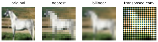
Figure 9.4. One CIFAR-10 test image (32 by 32 pixels) and the three simulated fakes made from it in Lab 9. Each fake halves the resolution by averaging 2-by-2 blocks and then enlarges the image again, with nearest-neighbor interpolation (blocky), bilinear interpolation (smooth) or a stride-2 transposed convolution with a fixed random 3-by-3 kernel (a strong checkerboard texture, the effect described by Odena et al.). The images are shown enlarged.
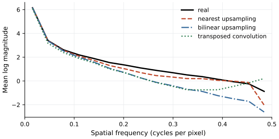
Figure 9.5. Mean azimuthally averaged log-magnitude spectra, equation \eqref{eq:azimuthal}, of 1,000 real CIFAR-10 test images and of the fakes from each simulated generator in Lab 9, computed on gray-scale images with 16 rings of equal width from zero frequency to the Nyquist frequency of 0.5 cycles per pixel; the last ring also collects the corners of the spectrum beyond 0.5 cycles per pixel. Averaged over rings 9 to 14 (0.25 to about 0.44 cycles per pixel), all three kinds of fake have a lower mean log magnitude than real images. In the last ring, bilinear fakes fall well below real images. Nearest-neighbor fakes fall below them as well, but only because their spectrum is exactly zero at the frequencies with a horizontal or vertical component of 0.5 cycles per pixel, where \(\epsilon\) sets the logarithm to about \(-6.9\); their mean power in the last ring is higher than that of real images. The transposed convolution leaves a higher mean log magnitude than real images in the last two rings.
Learned detectors
The alternative is to let a network learn whatever separates real from fake. FaceForensics++ (Rössler et al., 2019) provided a dataset of 1,000 original videos, each manipulated with four methods, and compared detectors on face crops. An XceptionNet pretrained on ImageNet reached binary accuracy of 99.26% on uncompressed videos, 95.73% on videos with light H.264 compression (quantization parameter 23) and 81.00% with strong compression (quantization parameter 40), while a detector built on hand-crafted steganalysis features fell from 97.63% to 55.98% over the same range. Compression hurt hand-crafted features and shallow networks most, and Rössler et al. attribute the better performance of XceptionNet to its ImageNet pretraining and larger capacity.
Wang et al. (2020) asked whether a detector trained on one generator could detect images from others. They trained a ResNet-50 classifier on images from ProGAN alone, with augmentation by blurring and JPEG compression, and tested it on images from eleven CNN-based generators, including StyleGAN, BigGAN, CycleGAN and a deepfake dataset. It generalized well to many of them, and augmentation raised the average precision on BigGAN images from 72.2 to 88.2. Augmentation also lowered performance on two test sets, the images of a super-resolution model whose traces are mainly high-frequency and the deepfake set, so it is a trade-off rather than a free gain.
Published detectors range from convolutional networks trained on real and generated images, like the one of Wang et al., to classifiers on the features of large pretrained models such as CLIP, which was trained on 400 million image and text pairs (Radford et al., 2021). Their reported accuracy depends on the generators and processing conditions used in training and testing, which is the subject of the next two sections.
The generalization gap
Detectors do well on the methods they were trained on and much worse on others. Two benchmarks quantify the gap for face-swap video. In Celeb-DF, Li et al. (2020) evaluated published detectors on several datasets. An XceptionNet trained on FaceForensics++ with light compression had a frame-level area under the ROC curve (AUC) of 99.7% on the FaceForensics++ deepfakes, 85.9% on Google's DeepFake Detection dataset, 72.2% on the preview DeepFake Detection Challenge (DFDC) data and 65.3% on Celeb-DF, whose deepfakes have fewer visible artifacts. The DFDC (Dolhansky et al., 2020) ranked submissions on a private test set that included deepfake videos found on the internet. The top five models had log losses between 0.17 and 0.22 on test videos made like the training data and between 0.66 and 0.70 on the real-world videos, close to the 0.69 of a detector that always outputs 0.5. Ranked by their scores, the real-world videos were separated better than chance, with an average precision of 0.753 and an ROC AUC of 0.734 for the best models, which the authors present as evidence that training on the DFDC data transfers to real videos.
Ojha et al. (2023) studied the same problem across generator families and explained one mechanism behind it. A classifier trained on real images and GAN images learns what GAN fakes look like, and its "real" class becomes a sink for everything else, including images from diffusion models it never saw. Their remedy was to avoid learning the real-versus-fake features at all. They used the frozen features of a CLIP vision transformer (ViT-L/14) with a nearest-neighbor or linear classifier trained on ProGAN data. On unseen diffusion and autoregressive models, they improved on the detector of Wang et al. by about 15 points of mean average precision with nearest-neighbor classification and about 19.5 points with the linear classifier.
Lab 9 reproduces the gap on a small scale. It trains two kinds of detector, a logistic regression on the 16 ring values of \eqref{eq:azimuthal} (the spectral detector) and a small convolutional network (CNN) on the pixels, each on real images against the fakes of one simulated generator. Figure 9.6 shows the AUC of each detector tested on all three generators. On the diagonal, every detector is close to perfect; the lowest diagonal AUC is 0.999 for the spectral detectors and 0.994 for the CNNs. Off the diagonal, results range from good to far below 0.5. The CNN trained on nearest-neighbor fakes ranks bilinear fakes above real images with AUC 0.979, although at its threshold of 0.5 it flags a share of only 0.019 of them, while the CNN trained on bilinear fakes reaches only 0.617 on nearest-neighbor fakes and 0.0003 on transposed-convolution fakes.
An AUC near zero does not mean that the score is random. It means that the detector ranks almost every one of those fakes as more real than almost every real photograph, so its score separates the two classes nearly perfectly but in the wrong direction. At its threshold of 0.5, the share of these fakes that it flags is 0.000. Reversing the score would help only someone who already had labeled fakes from the new generator, and the reversed detector would then fail on the generator it was trained on. The likely reason for the inversion, consistent with the spectra in Figure 9.5, is that the CNN learned weak high frequencies, which bilinear fakes show in every ring of the upper half of the band, as the sign of a fake, while the transposed convolution leaves more energy than real images in the highest ring. This is the sink-class effect in its simplest form. The spectral detector trained on nearest-neighbor fakes shows the same inversion less strongly (AUC 0.064); it relies mostly on a low mean log magnitude in the last ring, which for nearest-neighbor fakes comes from the exact zeros rather than from weak energy, and transposed-convolution fakes are higher than real images there. The spectral detector trained on bilinear fakes, by contrast, detects transposed-convolution fakes almost perfectly (AUC 0.9998), consistent with the spectra, in which both kinds of fake have a lower mean log magnitude than real images in each of rings 9 to 14. Which trace a detector picks up depends on the model as well as on the training data.
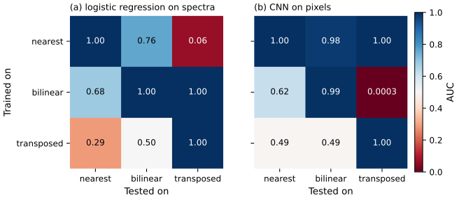
Figure 9.6. Generalization matrices from Lab 9. Each cell is the AUC of a detector trained on real images against fakes from the generator of its row and tested on real images against fakes from the generator of its column, on 1,000 real and 1,000 fake test images. (a) Logistic regression on the 16-value spectra of equation \eqref{eq:azimuthal}. (b) A small convolutional network on the pixels. An AUC of 0.5 (white) means that the score ranks fakes and real images at random. Blue cells are above 0.5, and red cells are below it, where the detector scores the unseen fakes as more real than the real images; an AUC near 0 is a nearly perfect ranking in the wrong direction.
Show the answer
First, which manipulation methods and which data were in training and in testing. An AUC measured on the same methods and source videos as the training data is an in-distribution number, and Celeb-DF and the DFDC show drops to an AUC near 0.65 or a log loss near chance when methods and sources change. Second, at what compression and resolution it was measured. FaceForensics++ results fall sharply from uncompressed to strongly compressed video, and video-call streams are compressed. A useful report states the generators and compression levels at test time and gives results on methods the detector was not trained on.
Compression and resizing
Compression and resizing are the normal life of shared media, and they act on the same high frequencies where many fingerprints live. The FaceForensics++ results above show the effect for video, and Celeb-DF confirms it. In Celeb-DF, the four strongest detectors lost between 4.7 and 17.4 points of AUC under strong H.264 compression (quantization parameter 40); the two XceptionNet detectors trained on compressed FaceForensics++ video kept their AUC at the light compression of quantization parameter 23 but not at strong compression (Li et al., 2020). Lab 9 compresses every test image with JPEG at quality 75 and tests the in-distribution detectors again. The spectral detector trained on nearest-neighbor fakes keeps an AUC of 0.971, but at its original threshold the share of fakes it flags falls from 1.000 to 0.005. The detector relied mainly on the low mean log magnitude of the last ring. JPEG compression puts nonzero values at the frequencies of 0.5 cycles per pixel where the spectrum of the nearest-neighbor fakes was exactly zero, which raises the mean log magnitude of their last ring close to that of compressed real images, as the lab prints. Their scores therefore drop below the threshold while still mostly exceeding the scores of real images. The other detectors are hardly affected in this simulation, whose fingerprints span whole bands of frequencies; the FaceForensics++ and Celeb-DF results show larger losses for real manipulation methods. The lesson for deployment is that a detector's threshold must be set on data processed the way deployment data is processed, and its AUC on clean data says little about its alert rate on recompressed uploads.
Adversarial attacks on detectors
A detector deployed against an adversary is a target for evasion, and the methods of Unit 7 apply directly. Carlini and Farid (2020) attacked a detector that achieved an AUC of 0.95 across many generators when trained on one. With full access to the classifier, flipping the lowest bit of each pixel reduced its AUC to 0.0005; perturbing 1% of the image area reduced it to 0.08; and a black-box attack with no access to the classifier reduced it to 0.22. The lowest-bit perturbation is invisible, and the universal patch is a small visible noise pattern in one corner of the image. The attacker faces fewer problem-space constraints than when evading a malware detector, since almost any pixel change that keeps the image looking the same serves its purpose. A detector's published accuracy is measured without an adversary, and these results show how far it can fall against someone who optimizes against it.
Audio deepfakes
Speech has its own benchmark series. ASVspoof, the spoofing and deepfake detection challenge, evaluates countermeasures that distinguish genuine (bona fide) speech from synthesized or converted speech. The 2021 edition (Liu et al., 2023) received evaluation submissions from 54 teams in three tasks. The logical access task concerns synthetic speech presented to an automatic speaker verification system, now transmitted over telephony and voice-over-IP channels with several codecs. The physical access task concerns replayed recordings. The new deepfake task concerns compressed speech posted online, without a speaker verification system. The main metric for the deepfake task is the equal error rate, the error rate at the threshold where the false acceptance and false rejection rates are equal. The organizers reported that logical access countermeasures were robust to the new encoding and transmission effects, and that deepfake countermeasures showed some resilience to compression but lacked generalization across different source datasets, the same pattern as for video.
How often a detector is right
The base rate is the last problem and often the decisive one. The DFDC authors note that in realistic traffic the ratio of deepfake videos to real ones may be less than one in a million, and that precision is then the most informative metric (Dolhansky et al., 2020). Take a detector with a true positive rate of 0.9 and a false positive rate of 0.01, better than most of the cross-dataset results above, and a base rate of one in a million. By Bayes' rule as in Lesson 1.2, its precision is
so about one alert in 11,000 is real. Screening everything with a detector is therefore impractical; detection is useful where the base rate is much higher, for example for content already reported as suspicious, or for the media attached to a payment request.
Show the answer
The base rate is \(\pi = 0.002\), and precision is
so about one flagged submission in fifteen is synthetic, and 30% of synthetic submissions pass unflagged. The flags are useful for routing submissions to further checks (a second verification step, document review, a live call), not for rejecting customers automatically, and the detector cannot be the only control, because most attacks it misses will not be examined at all.
Summary
Detectors of synthetic media exploit traces of the generation process, either known artifacts such as the spectral fingerprints of upsampling or patterns learned by a network from labeled examples, and both reach near-perfect accuracy on the methods they were trained on. Accuracy falls on unseen methods and datasets (an AUC of about 0.65 for a FaceForensics++ detector on Celeb-DF, a log loss near chance for the DFDC winners on real-world videos), in part because a detector learns what its training fakes look like and can treat everything else as real. Compression and resizing erase traces and shift scores, so thresholds must be set on realistically processed data. Detectors can be evaded by imperceptible perturbations, audio detectors face the same generalization problem, and at realistic base rates most alerts are false. Detection is one input among several, which is the starting point of Lesson 9.3.
References
- Carlini, N., and Farid, H. (2020). Evading deepfake-image detectors with white- and black-box attacks. 2020 IEEE/CVF Conference on Computer Vision and Pattern Recognition Workshops (CVPRW), 2804-2813. https://doi.org/10.1109/CVPRW50498.2020.00337
- Dolhansky, B., Bitton, J., Pflaum, B., Lu, J., Howes, R., Wang, M., and Canton Ferrer, C. (2020). The DeepFake Detection Challenge (DFDC) dataset. arXiv. arXiv preprint arXiv:2006.07397. https://arxiv.org/abs/2006.07397
- Durall, R., Keuper, M., and Keuper, J. (2020). Watch your up-convolution: CNN based generative deep neural networks are failing to reproduce spectral distributions. 2020 IEEE/CVF Conference on Computer Vision and Pattern Recognition (CVPR), 7887-7896. https://doi.org/10.1109/CVPR42600.2020.00791
- Frank, J., Eisenhofer, T., Schönherr, L., Fischer, A., Kolossa, D., and Holz, T. (2020). Leveraging frequency analysis for deep fake image recognition. Proceedings of the 37th International Conference on Machine Learning (ICML), PMLR, 119, 3247-3258. https://proceedings.mlr.press/v119/frank20a.html
- Li, Y., Yang, X., Sun, P., Qi, H., and Lyu, S. (2020). Celeb-DF: A large-scale challenging dataset for DeepFake forensics. 2020 IEEE/CVF Conference on Computer Vision and Pattern Recognition (CVPR), 3204-3213. https://doi.org/10.1109/CVPR42600.2020.00327
- Liu, X., Wang, X., Sahidullah, M., Patino, J., Delgado, H., Kinnunen, T., Todisco, M., Yamagishi, J., Evans, N., Nautsch, A., and Lee, K. A. (2023). ASVspoof 2021: Towards spoofed and deepfake speech detection in the wild. IEEE/ACM Transactions on Audio, Speech, and Language Processing, 31, 2507-2522. https://doi.org/10.1109/TASLP.2023.3285283
- Odena, A., Dumoulin, V., and Olah, C. (2016). Deconvolution and checkerboard artifacts. Distill, 1(10). https://doi.org/10.23915/distill.00003
- Ojha, U., Li, Y., and Lee, Y. J. (2023). Towards universal fake image detectors that generalize across generative models. 2023 IEEE/CVF Conference on Computer Vision and Pattern Recognition (CVPR), 24480-24489. https://doi.org/10.1109/CVPR52729.2023.02345
- Radford, A., Kim, J. W., Hallacy, C., Ramesh, A., Goh, G., Agarwal, S., Sastry, G., Askell, A., Mishkin, P., Clark, J., Krueger, G., and Sutskever, I. (2021). Learning transferable visual models from natural language supervision. Proceedings of the 38th International Conference on Machine Learning (ICML), PMLR, 139, 8748-8763. https://proceedings.mlr.press/v139/radford21a.html
- Rössler, A., Cozzolino, D., Verdoliva, L., Riess, C., Thies, J., and Nießner, M. (2019). FaceForensics++: Learning to detect manipulated facial images. 2019 IEEE/CVF International Conference on Computer Vision (ICCV), 1-11. https://doi.org/10.1109/ICCV.2019.00009
- Wang, S.-Y., Wang, O., Zhang, R., Owens, A., and Efros, A. A. (2020). CNN-generated images are surprisingly easy to spot ... for now. 2020 IEEE/CVF Conference on Computer Vision and Pattern Recognition (CVPR), 8692-8701. https://doi.org/10.1109/CVPR42600.2020.00872