Unit 9 · Lab 9
Generator fingerprints and the generalization gap
Lab 9
Generator fingerprints and the generalization gap
Open in ColabRead with outputsNotebook on GitHubAbout 2 minutes to run on a laptop CPU
# On Google Colab, install the scikit-learn version the course was built with.
# On your own computer, install requirements.txt instead; this cell then does nothing.
import subprocess, sys
if "google.colab" in sys.modules:
    subprocess.run([sys.executable, "-m", "pip", "install", "-q", "scikit-learn==1.9.0"], check=True)
Lab 9. Generator fingerprints and the generalization gap
This lab builds detectors of synthetic images and measures how well they transfer to a generation process they were not trained on. It runs in a few minutes on a laptop CPU.
The "fake" images here are not real deepfakes. They are CIFAR-10 photographs that were shrunk to half size and enlarged again by one of three upsampling operations, the building block that image generators use to go from a small internal representation to a full-size image. Each operation leaves its own trace in the frequency spectrum, which is the kind of trace that published detectors exploit (Lesson 9.2). We simulate generators this way for two reasons. Real deepfake datasets are tens to hundreds of gigabytes and are distributed under research licenses that require an application and forbid redistribution, so a self-contained lab cannot use them. And a controlled simulation lets us vary exactly one thing, the upsampling operation, so that the generalization gap we measure has a known cause. The lesson discusses what changes with real generators.
You will:
- create fake images with three simulated generators (nearest-neighbor upsampling, bilinear upsampling, and a stride-2 transposed convolution with a fixed random kernel);
- compute azimuthally averaged log-magnitude spectra and look at the average spectrum of each class;
- train a logistic-regression detector on spectra and a small convolutional network (CNN) on pixels, each on one generator, and test both on all three, giving two 3-by-3 generalization matrices;
- compress the test images with JPEG at quality 75 and measure the effect on detection, both on the ranking (AUC) and at a fixed threshold.
import io
import os
import time
import warnings

import numpy as np
import matplotlib.pyplot as plt
import torch
import torch.nn as nn
import torch.nn.functional as F
import torchvision
from PIL import Image
from sklearn.linear_model import LogisticRegression
from sklearn.metrics import roc_auc_score
from sklearn.pipeline import make_pipeline
from sklearn.preprocessing import StandardScaler

warnings.filterwarnings("ignore")
torch.manual_seed(0)
torch.set_num_threads(4)
t_start = time.time()

ROOT = "../../data/downloads"
os.makedirs(ROOT, exist_ok=True)
cifar_train = torchvision.datasets.CIFAR10(root=ROOT, train=True, download=True)
cifar_test = torchvision.datasets.CIFAR10(root=ROOT, train=False, download=True)

rng = np.random.default_rng(0)
N_TRAIN, N_TEST = 3000, 1000
tr = rng.choice(len(cifar_train), 2 * N_TRAIN, replace=False)
te = rng.choice(len(cifar_test), 2 * N_TEST, replace=False)
X_tr_all = cifar_train.data[tr].astype(np.float32) / 255.0      # (n, 32, 32, 3), values in [0, 1]
X_te_all = cifar_test.data[te].astype(np.float32) / 255.0
print(X_tr_all.shape, X_te_all.shape)
(6000, 32, 32, 3) (2000, 32, 32, 3)
1. Three simulated generators
Each simulated generator takes an image, averages it down to 16 by 16 pixels, and brings it back to 32 by 32 with a different upsampling operation:
nearestrepeats each pixel in a 2-by-2 block;bilinearinterpolates linearly between neighboring pixels;transposedapplies a stride-2 transposed convolution with a fixed random 3-by-3 kernel, as in many generator networks. Because the kernel size is not divisible by the stride, output pixels receive unequal numbers of contributions, and with a random kernel these contributions also have unequal weights. The result is the checkerboard pattern described by Odena et al. (2016).
Half of the images in each split are used as real images and the other half are turned into fakes, so that no fake has a real twin in the same split.
torch.manual_seed(1)
KERNEL = torch.rand(3, 1, 3, 3)                                  # one fixed random kernel per color channel
# kernel sum 4 matches the four output pixels per input pixel; the cropped border
# and the clamp to [0, 1] still make these fakes darker on average
KERNEL = KERNEL / KERNEL.sum(dim=(2, 3), keepdim=True) * 4


def generate(X, kind):
    x = torch.from_numpy(X).permute(0, 3, 1, 2)                  # (n, 3, 32, 32)
    small = F.avg_pool2d(x, 2)                                   # (n, 3, 16, 16)
    if kind == "nearest":
        y = F.interpolate(small, scale_factor=2, mode="nearest")
    elif kind == "bilinear":
        y = F.interpolate(small, scale_factor=2, mode="bilinear", align_corners=False)
    elif kind == "transposed":
        y = F.conv_transpose2d(small, KERNEL, stride=2, padding=1, output_padding=1, groups=3)
    else:
        raise ValueError(kind)
    return y.clamp(0, 1).permute(0, 2, 3, 1).numpy()


GENERATORS = ["nearest", "bilinear", "transposed"]
real_tr, base_tr = X_tr_all[:N_TRAIN], X_tr_all[N_TRAIN:]
real_te, base_te = X_te_all[:N_TEST], X_te_all[N_TEST:]
fake_tr = {g: generate(base_tr, g) for g in GENERATORS}
fake_te = {g: generate(base_te, g) for g in GENERATORS}

fig, axes = plt.subplots(1, 4, figsize=(8, 2.2))
for ax, (name, img) in zip(axes, [("original", base_te[0])] + [(g, fake_te[g][0]) for g in GENERATORS]):
    ax.imshow(img)
    ax.set_title(name)
    ax.axis("off")
plt.show()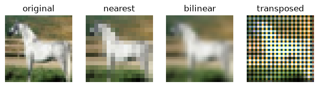
2. Azimuthally averaged spectra
For each image we take the gray-scale version, compute its two-dimensional discrete Fourier transform, and average the log magnitude over rings of equal distance from the zero frequency, as Durall et al. (2020) do with the power spectrum. Before taking the logarithm we add 0.001 to the magnitude, which keeps the logarithm finite where the magnitude is exactly zero, as happens for nearest-neighbor fakes. The result is a vector of 16 numbers, one per ring, with the rings running from zero frequency to the Nyquist frequency of half a cycle per pixel. The rings have equal width, and the last ring also collects the corners of the spectrum, whose frequencies reach about 0.71 cycles per pixel. Upsampling leaves its signature mainly at high frequencies.
N_BINS = 16
_fy, _fx = np.meshgrid(np.fft.fftfreq(32), np.fft.fftfreq(32), indexing="ij")
RADIUS = np.sqrt(_fx ** 2 + _fy ** 2)                           # cycles per pixel, 0 to about 0.71
BIN = np.minimum((RADIUS / 0.5 * N_BINS).astype(int), N_BINS - 1)
BIN_COUNT = np.bincount(BIN.ravel(), minlength=N_BINS)


def spectra(X):
    gray = X @ np.array([0.299, 0.587, 0.114], dtype=np.float32)
    logmag = np.log(np.abs(np.fft.fft2(gray)) + 1e-3)
    flat = logmag.reshape(len(X), -1)
    out = np.zeros((len(X), N_BINS))
    for b in range(N_BINS):
        out[:, b] = flat[:, BIN.ravel() == b].mean(axis=1)
    return out


S_real_tr, S_real_te = spectra(real_tr), spectra(real_te)
S_fake_tr = {g: spectra(fake_tr[g]) for g in GENERATORS}
S_fake_te = {g: spectra(fake_te[g]) for g in GENERATORS}
freq = (np.arange(N_BINS) + 0.5) / N_BINS * 0.5

fig, ax = plt.subplots(figsize=(6, 3.5))
ax.plot(freq, S_real_te.mean(0), "k-", label="real")
for g in GENERATORS:
    ax.plot(freq, S_fake_te[g].mean(0), label=g)
ax.set_xlabel("Spatial frequency (cycles per pixel)")
ax.set_ylabel("Mean log magnitude")
ax.legend()
plt.show()

print("mean log magnitude over test images")
for name, S in [("real", S_real_te)] + [(g, S_fake_te[g]) for g in GENERATORS]:
    print(f"{name:>11}: rings 9 to 14 {S[:, 8:14].mean():7.3f}   last ring {S[:, -1].mean():7.3f}")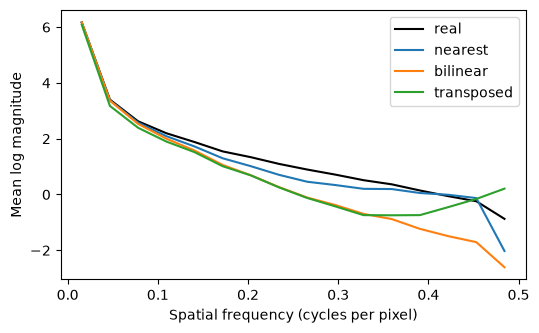
mean log magnitude over test images
       real: rings 9 to 14   0.428   last ring  -0.875
    nearest: rings 9 to 14   0.206   last ring  -2.027
   bilinear: rings 9 to 14  -0.799   last ring  -2.609
 transposed: rings 9 to 14  -0.539   last ring   0.209
Shrinking and enlarging removes detail, so on average over rings 9 to 14, which cover 0.25 to about 0.44 cycles per pixel, all three kinds of fake have less energy than real photographs. They differ in the last ring. Nearest-neighbor copies repeat each pixel in a 2-by-2 block, so the pixels come in equal pairs along each axis and the spectrum is exactly zero at the 63 frequencies of the last ring whose horizontal or vertical component is 0.5 cycles per pixel. The floor of 0.001 inside the logarithm turns these zeros into values of about -6.9, which pull the ring average far below that of real photographs, although the other 264 frequencies of the ring keep about as much magnitude as in real photographs. Bilinear interpolation suppresses the whole upper band more strongly, and the transposed convolution adds a periodic pattern that leaves more energy than real photographs in the last ring. The printed averages show both effects.
3. Detectors and the 3-by-3 generalization matrix
A detector is trained on real images against fakes from one generator and then tested on real images against fakes from each generator in turn. We report the area under the ROC curve (AUC) on the test images. The diagonal of the matrix is the usual in-distribution result; the off-diagonal entries measure generalization to a generator the detector never saw.
def labels(n_real, n_fake):
    return np.r_[np.zeros(n_real), np.ones(n_fake)]


auc_lr = np.zeros((3, 3))
lr_models = {}
for i, g_train in enumerate(GENERATORS):
    X = np.vstack([S_real_tr, S_fake_tr[g_train]])
    clf = make_pipeline(StandardScaler(), LogisticRegression(max_iter=2000)).fit(X, labels(N_TRAIN, N_TRAIN))
    lr_models[g_train] = clf
    for j, g_test in enumerate(GENERATORS):
        Xt = np.vstack([S_real_te, S_fake_te[g_test]])
        auc_lr[i, j] = roc_auc_score(labels(N_TEST, N_TEST), clf.predict_proba(Xt)[:, 1])
print("logistic regression on spectra, AUC (rows: trained on, columns: tested on)")
for i, g in enumerate(GENERATORS):
    print(f"{g:>11}: " + "  ".join(f"{v:.3f}" for v in auc_lr[i]))
logistic regression on spectra, AUC (rows: trained on, columns: tested on)
    nearest: 1.000  0.761  0.064
   bilinear: 0.683  0.999  1.000
 transposed: 0.288  0.498  1.000
Next we train a small CNN on the pixels themselves for a few epochs with Adam. It sees the raw images and can learn spatial patterns that the 16 ring averages do not capture, including ones that are specific to the generator it was trained on.
class SmallCNN(nn.Module):
    def __init__(self):
        super().__init__()
        self.c1 = nn.Conv2d(3, 16, 3, padding=1)
        self.c2 = nn.Conv2d(16, 32, 3, padding=1)
        self.f1 = nn.Linear(32 * 8 * 8, 64)
        self.f2 = nn.Linear(64, 1)

    def forward(self, x):
        x = F.max_pool2d(F.relu(self.c1(x)), 2)
        x = F.max_pool2d(F.relu(self.c2(x)), 2)
        return self.f2(F.relu(self.f1(x.flatten(1)))).squeeze(1)


def to_tensor(X):
    return torch.from_numpy(np.ascontiguousarray(X)).permute(0, 3, 1, 2).float()


def train_cnn(X, y, seed=0, epochs=6, batch=128):
    torch.manual_seed(seed)
    net = SmallCNN()
    opt = torch.optim.Adam(net.parameters(), lr=1e-3)
    Xt, yt = to_tensor(X), torch.from_numpy(y).float()
    g = torch.Generator().manual_seed(seed)
    for _ in range(epochs):
        perm = torch.randperm(len(Xt), generator=g)
        for k in range(0, len(Xt), batch):
            b = perm[k:k + batch]
            opt.zero_grad()
            F.binary_cross_entropy_with_logits(net(Xt[b]), yt[b]).backward()
            opt.step()
    net.eval()
    return net


def cnn_scores(net, X):
    with torch.no_grad():
        return torch.sigmoid(net(to_tensor(X))).numpy()


auc_cnn = np.zeros((3, 3))
cnn_models = {}
for i, g_train in enumerate(GENERATORS):
    net = train_cnn(np.concatenate([real_tr, fake_tr[g_train]]), labels(N_TRAIN, N_TRAIN))
    cnn_models[g_train] = net
    for j, g_test in enumerate(GENERATORS):
        s = cnn_scores(net, np.concatenate([real_te, fake_te[g_test]]))
        auc_cnn[i, j] = roc_auc_score(labels(N_TEST, N_TEST), s)
print("CNN on pixels, AUC (rows: trained on, columns: tested on)")
for i, g in enumerate(GENERATORS):
    print(f"{g:>11}: " + "  ".join(f"{v:.3f}" for v in auc_cnn[i]))
print(f"minutes so far: {(time.time() - t_start) / 60:.1f}")
CNN on pixels, AUC (rows: trained on, columns: tested on)
nearest: 1.000 0.979 1.000
bilinear: 0.617 0.994 0.000
transposed: 0.492 0.491 1.000
minutes so far: 0.4
fig, axes = plt.subplots(1, 2, figsize=(9, 3.6))
for ax, M, title in ((axes[0], auc_lr, "logistic regression on spectra"), (axes[1], auc_cnn, "CNN on pixels")):
    im = ax.imshow(M, vmin=0.0, vmax=1.0, cmap="RdBu")
    for i in range(3):
        for j in range(3):
            ax.text(j, i, f"{M[i, j]:.4f}" if M[i, j] < 0.005 else f"{M[i, j]:.2f}", ha="center", va="center",
                    color="white" if (M[i, j] > 0.85 or M[i, j] < 0.15) else "black")
    ax.set_xticks(range(3), GENERATORS)
    ax.set_yticks(range(3), GENERATORS)
    ax.set_xlabel("tested on")
    ax.set_ylabel("trained on")
    ax.set_title(title)
plt.tight_layout()
plt.show()

# share of the test fakes of each generator that each detector flags at the threshold 0.5
flag_lr, flag_cnn = np.zeros((3, 3)), np.zeros((3, 3))
for i, g_train in enumerate(GENERATORS):
    for j, g_test in enumerate(GENERATORS):
        flag_lr[i, j] = (lr_models[g_train].predict_proba(S_fake_te[g_test])[:, 1] >= 0.5).mean()
        flag_cnn[i, j] = (cnn_scores(cnn_models[g_train], fake_te[g_test]) >= 0.5).mean()
for name, M in (("logistic regression on spectra", flag_lr), ("CNN on pixels", flag_cnn)):
    print(f"{name}, share of fakes flagged at 0.5 (rows: trained on, columns: tested on)")
    for i, g in enumerate(GENERATORS):
        print(f"{g:>11}: " + "  ".join(f"{v:.3f}" for v in M[i]))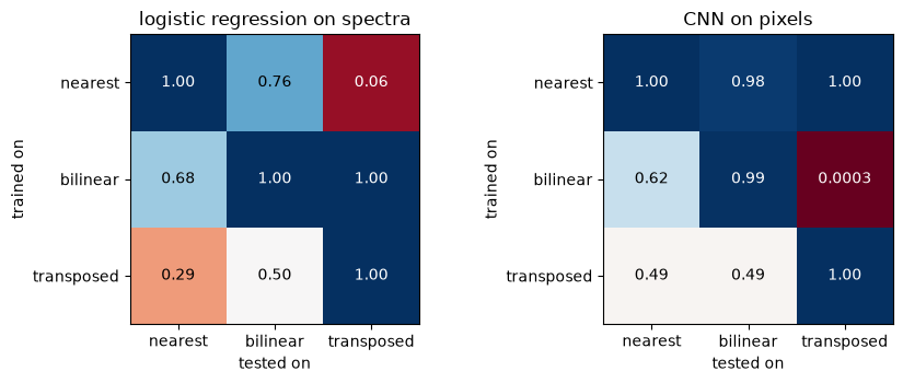
logistic regression on spectra, share of fakes flagged at 0.5 (rows: trained on, columns: tested on)
    nearest: 1.000  0.013  0.000
   bilinear: 0.034  0.993  0.999
 transposed: 0.000  0.000  1.000
CNN on pixels, share of fakes flagged at 0.5 (rows: trained on, columns: tested on)
    nearest: 1.000  0.019  1.000
   bilinear: 0.138  0.988  0.000
 transposed: 0.000  0.000  1.000
Read the matrices row by row. A detector can be nearly perfect on the generator it was trained on and much weaker on another one. The drop is not symmetric, since training on one generator may transfer to a second but not the other way round.
Some entries are far below 0.5. An AUC near 0 does not mean that the score is random. It means that the detector ranks almost every unseen fake as more real than almost every real photograph, so the score separates the two classes nearly perfectly but in the wrong direction. At the threshold of 0.5, the second printed table shows that such a detector flags almost none of these fakes. Reversing the score would require labeled fakes from the new generator, and the reversed detector would then fail on the generator it was trained on. The second table also shows that a high AUC off the diagonal does not mean that the new fakes are caught at the threshold. The CNN trained on nearest-neighbor fakes ranks bilinear fakes well above real images but flags few of them, because their scores, although higher than those of real images, mostly stay below 0.5.
The mean spectra above suggest the reason for the inversions. Nearest-neighbor and bilinear fakes have a lower mean log magnitude than real images in the last ring (for nearest-neighbor fakes because of the exact zeros at a horizontal or vertical frequency of 0.5 cycles per pixel), while transposed-convolution fakes have a higher one, so a detector that learned "weak high frequencies means fake" calls transposed-convolution fakes real. The spectral detector trained on bilinear fakes behaves differently from the CNN trained on the same fakes and flags almost all transposed-convolution fakes, which are also weak in rings 9 to 14. Which trace a detector picks up depends on the model as well as on the data. Lesson 9.2 relates these patterns to published results for real generators and manipulation methods.
4. JPEG compression
Images shared online are usually recompressed. JPEG discards high-frequency detail in 8-by-8 blocks, which is exactly where the fingerprints live, and it adds block artifacts of its own to real and fake images alike. We compress every test image, real and fake, with quality 75 and test the in-distribution detectors (the diagonal of each matrix) again, without retraining.
def jpeg(X, quality=75):
    out = np.empty_like(X)
    for k, img in enumerate(X):
        buf = io.BytesIO()
        Image.fromarray((img * 255).round().astype(np.uint8)).save(buf, format="JPEG", quality=quality)
        out[k] = np.asarray(Image.open(io.BytesIO(buf.getvalue())), dtype=np.float32) / 255.0
    return out


real_te_j = jpeg(real_te)
fake_te_j = {g: jpeg(fake_te[g]) for g in GENERATORS}
S_real_te_j = spectra(real_te_j)
y_test = labels(N_TEST, N_TEST)
jp = {}
for g in GENERATORS:
    s_lr = lr_models[g].predict_proba(np.vstack([S_real_te, S_fake_te[g]]))[:, 1]
    s_lr_j = lr_models[g].predict_proba(np.vstack([S_real_te_j, spectra(fake_te_j[g])]))[:, 1]
    s_cnn = cnn_scores(cnn_models[g], np.concatenate([real_te, fake_te[g]]))
    s_cnn_j = cnn_scores(cnn_models[g], np.concatenate([real_te_j, fake_te_j[g]]))
    for name, before, after in (("lr", s_lr, s_lr_j), ("cnn", s_cnn, s_cnn_j)):
        jp[(name, g)] = {
            "auc": roc_auc_score(y_test, after),
            "tpr": float((before[N_TEST:] >= 0.5).mean()), "tpr_jpeg": float((after[N_TEST:] >= 0.5).mean()),
            "fpr": float((before[:N_TEST] >= 0.5).mean()), "fpr_jpeg": float((after[:N_TEST] >= 0.5).mean()),
        }
    a, b = jp[("lr", g)], jp[("cnn", g)]
    print(f"{g:>11}: spectra AUC {a['auc']:.3f}, fakes flagged {a['tpr']:.3f} -> {a['tpr_jpeg']:.3f} | "
          f"CNN AUC {b['auc']:.3f}, fakes flagged {b['tpr']:.3f} -> {b['tpr_jpeg']:.3f}")

s_before = lr_models["nearest"].predict_proba(np.vstack([S_real_te, S_fake_te["nearest"]]))[:, 1]
s_after = lr_models["nearest"].predict_proba(np.vstack([S_real_te_j, spectra(fake_te_j["nearest"])]))[:, 1]
coef = lr_models["nearest"][-1].coef_[0]
print("spectral detector trained on nearest-neighbor fakes")
print("  standardized coefficients, rings 1 to 16:", " ".join(f"{c:.2f}" for c in coef))
print("before -> after JPEG")
print(f"  last ring, real images:   {S_real_te[:, -1].mean():7.3f} -> {S_real_te_j[:, -1].mean():7.3f}")
print(f"  last ring, nearest fakes: {S_fake_te['nearest'][:, -1].mean():7.3f} -> {spectra(fake_te_j['nearest'])[:, -1].mean():7.3f}")
print(f"  median score, real:  {np.median(s_before[:N_TEST]):.4f} -> {np.median(s_after[:N_TEST]):.4f}")
print(f"  median score, fakes: {np.median(s_before[N_TEST:]):.4f} -> {np.median(s_after[N_TEST:]):.4f}")
nearest: spectra AUC 0.971, fakes flagged 1.000 -> 0.005 | CNN AUC 1.000, fakes flagged 1.000 -> 0.999
bilinear: spectra AUC 0.999, fakes flagged 0.993 -> 0.994 | CNN AUC 0.992, fakes flagged 0.988 -> 0.983
 transposed: spectra AUC 1.000, fakes flagged 1.000 -> 1.000 | CNN AUC 1.000, fakes flagged 1.000 -> 1.000
spectral detector trained on nearest-neighbor fakes
  standardized coefficients, rings 1 to 16: -0.03 0.26 0.02 0.05 0.10 -0.17 -0.24 -0.82 -1.05 -0.80 -0.61 0.05 0.67 2.06 2.70 -6.24
before -> after JPEG
  last ring, real images:    -0.875 ->  -0.822
  last ring, nearest fakes:  -2.027 ->  -0.837
  median score, real:  0.0004 -> 0.0001
  median score, fakes: 0.9995 -> 0.0118
The first table gives, for each in-distribution detector, the AUC on compressed test images and the share of fakes flagged at the default threshold of 0.5 before and after compression. AUC measures only the ranking. A detector can keep most of its ranking and still miss most fakes at the threshold it was deployed with, which is what happens to the spectral detector trained on nearest-neighbor fakes. The last lines show why. The coefficient of the last ring is by far the largest in absolute value, and it is negative, so the detector reads a low mean log magnitude in that ring as the sign of a fake. JPEG compression puts nonzero values at the frequencies of 0.5 cycles per pixel where the spectrum of the nearest-neighbor fakes was exactly zero, and so raises the mean log magnitude of their last ring close to that of real images, while the rest of the ring changes little. As a result, the median score of the fakes drops below the threshold, while the scores of real images change little and stay lower still. In this simulation the other detectors are hardly affected, because the simulated fingerprints span whole bands of frequencies; for real manipulation methods, the published results in Lesson 9.2 show larger losses under compression.
Detectors trained only on uncompressed images see compressed inputs unlike anything in their training data. Wang et al. (2020) trained with blur and JPEG compression as augmentation and found that it improved detection on most of their test generators, though not on all; the first "Try this" item below lets you test the idea here.
Try this
- Apply
jpeg()to the training images as well and retrain the nearest-neighbor detectors. Predict which entries of the matrices improve. - Replace the 3-by-3 transposed-convolution kernel by a 4-by-4 kernel with
padding=1and nooutput_padding. The kernel size is then divisible by the stride, so every interior output pixel receives the same number of contributions. Before you run it, compute the sums of the four interleaved 2-by-2 sub-kernels (KERNEL[:, :, 0::2, 0::2]and so on) and predict whether the checkerboard disappears. - Train one detector on fakes from two generators and test it on the third. Does seeing more generators help?
Results summary
These are the numbers quoted in the lesson text.
results = {"n_train_real": N_TRAIN, "n_test_real": N_TEST, "minutes_total": float((time.time() - t_start) / 60)}
for i, a in enumerate(GENERATORS):
    for j, b in enumerate(GENERATORS):
        results[f"lr_{a}_{b}"] = float(auc_lr[i, j])
        results[f"cnn_{a}_{b}"] = float(auc_cnn[i, j])
    for name in ("lr", "cnn"):
        r = jp[(name, a)]
        results[f"{name}_jpeg_auc_{a}"] = float(r["auc"])
        results[f"{name}_tpr_{a}"] = r["tpr"]
        results[f"{name}_jpeg_tpr_{a}"] = r["tpr_jpeg"]
        results[f"{name}_fpr_{a}"] = r["fpr"]
        results[f"{name}_jpeg_fpr_{a}"] = r["fpr_jpeg"]
for i, a in enumerate(GENERATORS):
    for j, b in enumerate(GENERATORS):
        results[f"lr_flag_{a}_{b}"] = float(flag_lr[i, j])
        results[f"cnn_flag_{a}_{b}"] = float(flag_cnn[i, j])
results["lr_offdiag_min"] = float(min(auc_lr[i, j] for i in range(3) for j in range(3) if i != j))
results["cnn_offdiag_min"] = float(min(auc_cnn[i, j] for i in range(3) for j in range(3) if i != j))
results["lr_diag_min"] = float(np.diag(auc_lr).min())
results["cnn_diag_min"] = float(np.diag(auc_cnn).min())
export = {
    "generators": GENERATORS,
    "freq": freq.tolist(),
    "spectrum_real": S_real_te.mean(0).tolist(),
    **{f"spectrum_{g}": S_fake_te[g].mean(0).tolist() for g in GENERATORS},
    "spectrum_real_jpeg": S_real_te_j.mean(0).tolist(),
    **{f"spectrum_{g}_jpeg": spectra(fake_te_j[g]).mean(0).tolist() for g in GENERATORS},
    "auc_lr": auc_lr.tolist(),
    "auc_cnn": auc_cnn.tolist(),
    "auc_jpeg_lr": [float(jp[("lr", g)]["auc"]) for g in GENERATORS],
    "auc_jpeg_cnn": [float(jp[("cnn", g)]["auc"]) for g in GENERATORS],
    "tpr_lr": [jp[("lr", g)]["tpr"] for g in GENERATORS],
    "tpr_jpeg_lr": [jp[("lr", g)]["tpr_jpeg"] for g in GENERATORS],
    "tpr_cnn": [jp[("cnn", g)]["tpr"] for g in GENERATORS],
    "tpr_jpeg_cnn": [jp[("cnn", g)]["tpr_jpeg"] for g in GENERATORS],
    "example_original": (base_te[0] * 255).round().astype(int).tolist(),
    **{f"example_{g}": (fake_te[g][0] * 255).round().astype(int).tolist() for g in GENERATORS},
}
for k, v in results.items():
    print(f"{k:<28} {v}")

# When the course build runs this notebook, it saves the numbers for the lesson pages.
if os.environ.get("COURSE_RESULTS"):
    import json
    with open(os.environ["COURSE_RESULTS"], "w") as f:
        json.dump({"results": results, "data": export}, f)
n_train_real 3000 n_test_real 1000 minutes_total 0.4873330116271973 lr_nearest_nearest 1.0 cnn_nearest_nearest 0.999996 lr_nearest_bilinear 0.7609620000000001 cnn_nearest_bilinear 0.978673 lr_nearest_transposed 0.064239 cnn_nearest_transposed 1.0 lr_jpeg_auc_nearest 0.971243 lr_tpr_nearest 1.0 lr_jpeg_tpr_nearest 0.005 lr_fpr_nearest 0.0 lr_jpeg_fpr_nearest 0.0 cnn_jpeg_auc_nearest 0.999985 cnn_tpr_nearest 1.0 cnn_jpeg_tpr_nearest 0.999 cnn_fpr_nearest 0.002 cnn_jpeg_fpr_nearest 0.002 lr_bilinear_nearest 0.683444 cnn_bilinear_nearest 0.616915 lr_bilinear_bilinear 0.999321 cnn_bilinear_bilinear 0.9941359999999999 lr_bilinear_transposed 0.999772 cnn_bilinear_transposed 0.00026500000000000004 lr_jpeg_auc_bilinear 0.999123 lr_tpr_bilinear 0.993 lr_jpeg_tpr_bilinear 0.994 lr_fpr_bilinear 0.015 lr_jpeg_fpr_bilinear 0.014 cnn_jpeg_auc_bilinear 0.992312 cnn_tpr_bilinear 0.988 cnn_jpeg_tpr_bilinear 0.983 cnn_fpr_bilinear 0.071 cnn_jpeg_fpr_bilinear 0.081 lr_transposed_nearest 0.288421 cnn_transposed_nearest 0.492002 lr_transposed_bilinear 0.498025 cnn_transposed_bilinear 0.490622 lr_transposed_transposed 1.0 cnn_transposed_transposed 1.0 lr_jpeg_auc_transposed 1.0 lr_tpr_transposed 1.0 lr_jpeg_tpr_transposed 1.0 lr_fpr_transposed 0.0 lr_jpeg_fpr_transposed 0.0 cnn_jpeg_auc_transposed 1.0 cnn_tpr_transposed 1.0 cnn_jpeg_tpr_transposed 1.0 cnn_fpr_transposed 0.0 cnn_jpeg_fpr_transposed 0.0 lr_flag_nearest_nearest 1.0 cnn_flag_nearest_nearest 1.0 lr_flag_nearest_bilinear 0.013 cnn_flag_nearest_bilinear 0.019 lr_flag_nearest_transposed 0.0 cnn_flag_nearest_transposed 1.0 lr_flag_bilinear_nearest 0.034 cnn_flag_bilinear_nearest 0.138 lr_flag_bilinear_bilinear 0.993 cnn_flag_bilinear_bilinear 0.988 lr_flag_bilinear_transposed 0.999 cnn_flag_bilinear_transposed 0.0 lr_flag_transposed_nearest 0.0 cnn_flag_transposed_nearest 0.0 lr_flag_transposed_bilinear 0.0 cnn_flag_transposed_bilinear 0.0 lr_flag_transposed_transposed 1.0 cnn_flag_transposed_transposed 1.0 lr_offdiag_min 0.064239 cnn_offdiag_min 0.00026500000000000004 lr_diag_min 0.999321 cnn_diag_min 0.9941359999999999