Unit 8 · Lab 8b
Membership inference and DP-SGD
Lab 8b
Membership inference and DP-SGD
Open in ColabRead with outputsNotebook on GitHubAbout 6 minutes to run on a laptop CPU
# On Google Colab, install the scikit-learn version the course was built with.
# On your own computer, install requirements.txt instead; this cell then does nothing.
import subprocess, sys
if "google.colab" in sys.modules:
    subprocess.run([sys.executable, "-m", "pip", "install", "-q", "scikit-learn==1.9.0"], check=True)
Lab 8b. Membership inference and DP-SGD
This lab measures how much a trained model reveals about whether a given record was in its training set, and how differentially private training limits that leak. It uses a subset of the MNIST handwritten digits, because membership inference is easiest to see on a model that can memorize individual examples, and it runs in a few minutes on a laptop CPU.
You will:
- split a pool of images at random into members (used for training) and non-members;
- train a small network until it overfits and run a loss-threshold membership inference attack, reporting the area under the ROC curve (AUC) and the true positive rate at false positive rates of 1% and 0.1%;
- run a stronger attack that calibrates each example's score with reference models;
- train the same network with DP-SGD, written out by hand, at three noise levels, compute the privacy parameter \(\epsilon\) with the Rényi differential privacy accountant (
RDPAccountant) of the Opacus library, and measure test accuracy and both attacks again.
The next cell installs Opacus if it is missing (it is not preinstalled on Colab). Opacus is used only for privacy accounting.
try:
    import opacus  # noqa: F401
except ImportError:
    %pip install -q opacus
import os
import time
import warnings
import numpy as np
import matplotlib.pyplot as plt
import torch
import torch.nn as nn
import torchvision
from opacus.accountants import RDPAccountant
from sklearn.metrics import roc_auc_score, roc_curve
warnings.filterwarnings("ignore")
torch.manual_seed(0)
torch.set_num_threads(2) # the networks are small; more threads only add overhead
t_start = time.time()
ROOT = "../../data/downloads"
os.makedirs(ROOT, exist_ok=True)
train_set = torchvision.datasets.MNIST(root=ROOT, train=True, download=True)
test_set = torchvision.datasets.MNIST(root=ROOT, train=False, download=True)
def prepare(ds):
X = ds.data.float().div(255).view(-1, 784)
return (X - 0.1307) / 0.3081, ds.targets.clone()
X_all, Y_all = prepare(train_set)
X_test, Y_test = prepare(test_set)1. Members and non-members
We draw a pool of 4,000 training images and flip a fair coin for each one. Heads, the image is a member and is used to train the target model; tails, it is a non-member. The attacker sees an image and the model, and must decide which. Because membership was decided by a coin, an attacker who knows nothing has an AUC of 0.5 and a true positive rate equal to its false positive rate.
POOL = 4_000
rng = np.random.default_rng(0)
pool_idx = rng.choice(len(X_all), POOL, replace=False)
X_pool, Y_pool = X_all[pool_idx], Y_all[pool_idx]
member = rng.random(POOL) < 0.5
X_tr, Y_tr = X_pool[member], Y_pool[member]
print(f"members: {member.sum():,}, non-members: {(~member).sum():,}")
members: 1,999, non-members: 2,001
2. An overfit model and the loss-threshold attack
The target model is a multilayer perceptron with one hidden layer of 256 units, trained with Adam for 60 epochs and no regularization, long enough to classify every training image correctly.
HIDDEN = 256


def make_net(seed):
    torch.manual_seed(seed)
    return nn.Sequential(nn.Linear(784, HIDDEN), nn.ReLU(), nn.Linear(HIDDEN, 10))


def train_adam(X, Y, seed, epochs=60, batch=128):
    net = make_net(seed)
    opt = torch.optim.Adam(net.parameters(), lr=1e-3)
    g = torch.Generator().manual_seed(seed)
    for _ in range(epochs):
        perm = torch.randperm(len(X), generator=g)
        for i in range(0, len(X), batch):
            b = perm[i:i + batch]
            opt.zero_grad()
            nn.functional.cross_entropy(net(X[b]), Y[b]).backward()
            opt.step()
    return net


def accuracy(net, X, Y):
    with torch.no_grad():
        return (net(X).argmax(1) == Y).float().mean().item()


target = train_adam(X_tr, Y_tr, seed=1)
acc_train, acc_test = accuracy(target, X_tr, Y_tr), accuracy(target, X_test, Y_test)
print(f"train accuracy {acc_train:.4f}, test accuracy {acc_test:.4f}")
train accuracy 1.0000, test accuracy 0.9227
The attack of Yeom et al. (2018) predicts "member" when the model's loss on the example is below a threshold. We use an equivalent score that does not lose precision when the loss is tiny, the logit-scaled confidence \(\log\big(p_y/(1-p_y)\big)\), where \(p_y\) is the probability the model gives the true label (Carlini et al., 2022). The cross-entropy loss is \(-\log p_y\), so a high score is the same as a low loss, and a threshold on one is a threshold on the other.
def membership_score(net, X, Y):
    """log(p_y / (1 - p_y)), computed from the logits in float64."""
    with torch.no_grad():
        z = net(X).double()
    rows = torch.arange(len(Y))
    z_true = z[rows, Y]
    z_other = z.clone()
    z_other[rows, Y] = -float("inf")
    return (z_true - torch.logsumexp(z_other, dim=1)).numpy()


def attack_metrics(score, is_member):
    fpr, tpr, _ = roc_curve(is_member, score)

    def tpr_at(f):
        return float(tpr[np.searchsorted(fpr, f, side="right") - 1])

    return {"auc": float(roc_auc_score(is_member, score)), "tpr_1": tpr_at(0.01), "tpr_01": tpr_at(0.001),
            "fpr": fpr, "tpr": tpr}


def intervals(score, is_member, n_boot=1000, seed=0):
    """95% bootstrap intervals for the AUC and the TPR at FPR 1% and 0.1%, resampling members and non-members separately."""
    rng_b = np.random.default_rng(seed)
    m_idx, n_idx = np.flatnonzero(is_member), np.flatnonzero(~is_member)
    stats = []
    for _ in range(n_boot):
        idx = np.concatenate([rng_b.choice(m_idx, len(m_idx)), rng_b.choice(n_idx, len(n_idx))])
        a = attack_metrics(score[idx], is_member[idx])
        stats.append((a["auc"], a["tpr_1"], a["tpr_01"]))
    lo, hi = np.percentile(np.array(stats), [2.5, 97.5], axis=0)
    return {"auc": (lo[0], hi[0]), "tpr_1": (lo[1], hi[1]), "tpr_01": (lo[2], hi[2])}


def show(name, att, ci):
    print(f"{name}: AUC {att['auc']:.3f} [{ci['auc'][0]:.3f}, {ci['auc'][1]:.3f}], "
          f"TPR at 1% FPR {att['tpr_1']:.4f} [{ci['tpr_1'][0]:.4f}, {ci['tpr_1'][1]:.4f}], "
          f"TPR at 0.1% FPR {att['tpr_01']:.4f} [{ci['tpr_01'][0]:.4f}, {ci['tpr_01'][1]:.4f}]")


score_target = membership_score(target, X_pool, Y_pool)
loss_attack = attack_metrics(score_target, member)
loss_ci = intervals(score_target, member)
show("loss-threshold attack", loss_attack, loss_ci)
print(f"balanced attack accuracy of the best threshold: {0.5 + 0.5 * np.max(loss_attack['tpr'] - loss_attack['fpr']):.3f}")
loss-threshold attack: AUC 0.571 [0.553, 0.589], TPR at 1% FPR 0.0065 [0.0015, 0.0120], TPR at 0.1% FPR 0.0000 [0.0000, 0.0025] balanced attack accuracy of the best threshold: 0.616
The numbers in brackets are 95% intervals from a bootstrap that resamples the members and the non-members of the pool. They show how much each number depends on which records happened to be evaluated; they do not include the variation from retraining the target model.
The AUC is above 0.5, so the model leaks membership on average. The true positive rate at a false positive rate of 0.1% is the more telling number. It answers the question that matters to a person whose record might be in the training set, whether an attacker can identify some members with confidence. A global loss threshold does poorly there, because many non-members are easy images that any model classifies with tiny loss, and they are indistinguishable from members by loss alone.
3. Calibrating each example with reference models
Carlini et al. (2022) showed that the attack becomes much stronger at low false positive rates when each example's score is compared with how that same example scores on models that did not train on it. We train 16 reference models, each on a random half of the pool, with the same training procedure as the target. For every image, about eight reference models did not see it; the mean and standard deviation of its score on those models describe how confident a model is on that image when it is not a member. The calibrated score is the target score minus that mean, divided by that standard deviation. This is a simplified form of the offline variant of their likelihood ratio attack. It assumes the attacker knows the training procedure and has data from the same distribution, which Lesson 8.2 discusses.
K = 16


def calibrated_scores(score, train_fn, seed0, k_ref=K):
    """Standardize each example's target score by its scores on reference models that did not train on it."""
    ref = np.zeros((k_ref, POOL))
    out = np.zeros((k_ref, POOL), dtype=bool)
    for k in range(k_ref):
        in_k = np.random.default_rng(seed0 + k).random(POOL) < 0.5
        ref[k] = membership_score(train_fn(X_pool[in_k], Y_pool[in_k], seed0 + k), X_pool, Y_pool)
        out[k] = ~in_k
    cnt = out.sum(0)
    mu = (ref * out).sum(0) / np.maximum(cnt, 1)
    var = (((ref - mu) ** 2) * out).sum(0) / np.maximum(cnt - 1, 1)
    return (score - mu) / np.sqrt(np.maximum(var, 1e-2))


cal_score = calibrated_scores(score_target, train_adam, seed0=100)
cal_attack = attack_metrics(cal_score, member)
cal_ci = intervals(cal_score, member)
show("calibrated attack", cal_attack, cal_ci)
print(f"minutes so far: {(time.time() - t_start) / 60:.1f}")
calibrated attack: AUC 0.633 [0.616, 0.650], TPR at 1% FPR 0.0720 [0.0555, 0.0906], TPR at 0.1% FPR 0.0130 [0.0030, 0.0530] minutes so far: 1.1
fig, ax = plt.subplots(figsize=(5, 4.2))
ax.plot(loss_attack["fpr"], loss_attack["tpr"], label=f"loss threshold (AUC {loss_attack['auc']:.2f})")
ax.plot(cal_attack["fpr"], cal_attack["tpr"], label=f"calibrated (AUC {cal_attack['auc']:.2f})")
ax.plot([1e-4, 1], [1e-4, 1], "k:", label="chance")
ax.set_xscale("log")
ax.set_yscale("log")
ax.set_xlim(1e-4, 1)
ax.set_ylim(1e-4, 1)
ax.set_xlabel("False positive rate")
ax.set_ylabel("True positive rate")
ax.legend()
plt.show()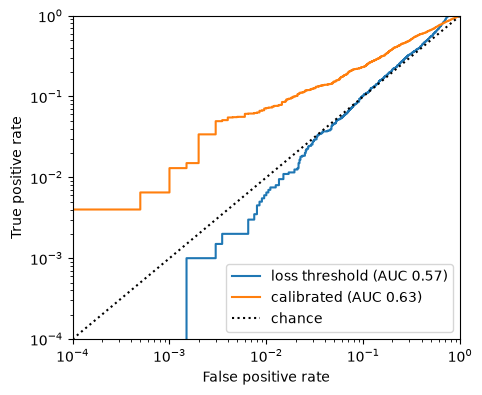
On log axes, the region that matters (false positive rates of 1% and below) is visible. On linear axes, both curves would look close to the diagonal. With 2,000 or so non-members, a false positive rate of 0.1% corresponds to about two non-members, so the numbers at that rate are noisy, which is why their intervals printed above are wide. A reliable measurement at a false positive rate of 0.1% needs many thousands of non-members.
4. DP-SGD by hand
DP-SGD (Abadi et al., 2016) changes one step of ordinary minibatch training. Each example's gradient is clipped to Euclidean norm at most \(C\), the clipped gradients are summed, Gaussian noise with standard deviation \(\sigma C\) is added to the sum, where \(\sigma\) is the noise multiplier, and the result is divided by the expected batch size. The batch is formed by Poisson sampling, each example joining independently with probability \(q\), which is what the privacy accountant assumes.
Per-example gradients are cheap for a network made of dense layers. For a layer with input \(a\) and gradient \(u\) with respect to its output, the per-example weight gradient is the outer product \(a\,u^\top\), whose Frobenius norm is \(\lVert a\rVert\,\lVert u\rVert\). The function below uses this to compute every example's full gradient norm without forming the gradients, and then forms only the clipped sum.
class DPMLP:
    """The same one-hidden-layer network, with weights held as plain tensors."""

    def __init__(self, seed):
        net = make_net(seed)
        self.W1 = net[0].weight.detach().T.clone()
        self.b1 = net[0].bias.detach().clone()
        self.W2 = net[2].weight.detach().T.clone()
        self.b2 = net[2].bias.detach().clone()

    def __call__(self, X):
        return torch.relu(X @ self.W1 + self.b1) @ self.W2 + self.b2

    def params(self):
        return [self.W1, self.b1, self.W2, self.b2]


def clipped_gradient_sum(m, X, Y, C):
    """Sum over the batch of per-example gradients, each clipped to norm C."""
    a = torch.relu(X @ m.W1 + m.b1)
    p = torch.softmax(a @ m.W2 + m.b2, dim=1)
    d2 = p.clone()
    d2[torch.arange(len(Y)), Y] -= 1.0                 # gradient of the loss w.r.t. the logits
    d1 = (d2 @ m.W2.T) * (a > 0)                       # w.r.t. the hidden pre-activations
    sq_norm = (d1 ** 2).sum(1) * ((X ** 2).sum(1) + 1) + (d2 ** 2).sum(1) * ((a ** 2).sum(1) + 1)
    scale = (C / (sq_norm.sqrt() + 1e-12)).clamp(max=1.0)
    d1s, d2s = d1 * scale[:, None], d2 * scale[:, None]
    return [X.T @ d1s, d1s.sum(0), a.T @ d2s, d2s.sum(0)], sq_norm.sqrt()


# Check the per-example norms against autograd on a few examples.
m_check = DPMLP(seed=5)
_, norms = clipped_gradient_sum(m_check, X_tr[:4], Y_tr[:4], C=1e9)
for i in range(4):
    ps = [p.clone().requires_grad_(True) for p in m_check.params()]
    out = torch.relu(X_tr[i:i + 1] @ ps[0] + ps[1]) @ ps[2] + ps[3]
    gs = torch.autograd.grad(nn.functional.cross_entropy(out, Y_tr[i:i + 1]), ps)
    print(f"example {i}: closed form {norms[i]:.5f}, autograd {torch.sqrt(sum((g ** 2).sum() for g in gs)):.5f}")
example 0: closed form 12.88036, autograd 12.88036 example 1: closed form 13.89285, autograd 13.89285 example 2: closed form 14.61452, autograd 14.61451 example 3: closed form 10.34340, autograd 10.34340
The training loop follows. With \(\sigma = 0\) it is clipped minibatch SGD with Poisson sampling and no noise, which we also run as a reference, with the same algorithm and the same number of steps but no privacy guarantee. For each setting we run both attacks; the calibrated attack trains its reference models with the same algorithm and noise level as the target, again with 16 reference models.
Q = 0.05          # sampling probability: expected batch of about 100 members
STEPS = 300       # 15 epochs
CLIP = 1.0
LR = 1.0
DELTA = 1e-5


def train_dpsgd(X, Y, sigma, seed=0):
    m = DPMLP(seed)
    g = torch.Generator().manual_seed(seed + 1)
    n = len(X)
    for _ in range(STEPS):
        idx = torch.nonzero(torch.rand(n, generator=g) < Q).squeeze(1)
        if len(idx) == 0:
            continue
        grads, _ = clipped_gradient_sum(m, X[idx], Y[idx], CLIP)
        for P, G in zip(m.params(), grads):
            noise = sigma * CLIP * torch.randn(G.shape, generator=g) if sigma > 0 else 0.0
            P -= LR * (G + noise) / (Q * n)
    return m


def epsilon(sigma):
    acc = RDPAccountant()
    acc.history = [(sigma, Q, STEPS)]
    return float(acc.get_epsilon(delta=DELTA))


K_DP = 16         # reference models per setting, as for the target
runs = {}
for sigma in (0.0, 0.6, 1.0, 3.0):
    m = train_dpsgd(X_tr, Y_tr, sigma)
    s = membership_score(m, X_pool, Y_pool)
    loss_att = attack_metrics(s, member)
    s_cal = calibrated_scores(s, lambda X, Y, seed: train_dpsgd(X, Y, sigma, seed), seed0=200, k_ref=K_DP)
    cal_att = attack_metrics(s_cal, member)
    runs[sigma] = {"eps": epsilon(sigma) if sigma > 0 else float("inf"), "acc_test": accuracy(m, X_test, Y_test),
                   "loss": loss_att, "cal": cal_att, "loss_ci": intervals(s, member), "cal_ci": intervals(s_cal, member)}
    r = runs[sigma]
    print(f"sigma {sigma:.1f}: epsilon {r['eps']:.2f}, test accuracy {r['acc_test']:.3f}")
    show("  loss-threshold attack", loss_att, r["loss_ci"])
    show("  calibrated attack", cal_att, r["cal_ci"])
print(f"minutes so far: {(time.time() - t_start) / 60:.1f}")
sigma 0.0: epsilon inf, test accuracy 0.901 loss-threshold attack: AUC 0.545 [0.527, 0.562], TPR at 1% FPR 0.0095 [0.0035, 0.0160], TPR at 0.1% FPR 0.0005 [0.0000, 0.0030] calibrated attack: AUC 0.603 [0.586, 0.621], TPR at 1% FPR 0.0340 [0.0180, 0.0550], TPR at 0.1% FPR 0.0110 [0.0040, 0.0195]
sigma 0.6: epsilon 21.02, test accuracy 0.867
  loss-threshold attack: AUC 0.535 [0.516, 0.553], TPR at 1% FPR 0.0055 [0.0025, 0.0105], TPR at 0.1% FPR 0.0005 [0.0000, 0.0045]
  calibrated attack: AUC 0.550 [0.533, 0.568], TPR at 1% FPR 0.0110 [0.0035, 0.0220], TPR at 0.1% FPR 0.0005 [0.0000, 0.0020]
sigma 1.0: epsilon 6.46, test accuracy 0.803
  loss-threshold attack: AUC 0.529 [0.512, 0.547], TPR at 1% FPR 0.0090 [0.0040, 0.0145], TPR at 0.1% FPR 0.0010 [0.0000, 0.0030]
  calibrated attack: AUC 0.535 [0.518, 0.551], TPR at 1% FPR 0.0070 [0.0035, 0.0160], TPR at 0.1% FPR 0.0010 [0.0000, 0.0045]
sigma 3.0: epsilon 1.27, test accuracy 0.586
  loss-threshold attack: AUC 0.519 [0.502, 0.538], TPR at 1% FPR 0.0135 [0.0080, 0.0200], TPR at 0.1% FPR 0.0010 [0.0000, 0.0040]
  calibrated attack: AUC 0.516 [0.498, 0.534], TPR at 1% FPR 0.0090 [0.0050, 0.0190], TPR at 0.1% FPR 0.0005 [0.0000, 0.0025]
minutes so far: 3.3
For an \((\epsilon, \delta)\)-differentially private training algorithm, no attack can have a true positive rate above \(e^{\epsilon}\cdot\mathrm{FPR} + \delta\) in the game where each candidate record is included at random (Lesson 8.3). The next cell evaluates that ceiling at the two false positive rates. When \(\epsilon\) is large the ceiling exceeds 1 and says nothing; when \(\epsilon\) is small it is a real guarantee that holds for every attack, including attacks not yet invented.
for sigma in (0.6, 1.0, 3.0):
    e = runs[sigma]["eps"]
    print(f"epsilon {e:5.2f}: TPR ceiling at 1% FPR {min(1, np.exp(e) * 0.01 + DELTA):.4f}, "
          f"at 0.1% FPR {min(1, np.exp(e) * 0.001 + DELTA):.4f}; measured (calibrated) "
          f"{runs[sigma]['cal']['tpr_1']:.4f} and {runs[sigma]['cal']['tpr_01']:.4f}")
epsilon 21.02: TPR ceiling at 1% FPR 1.0000, at 0.1% FPR 1.0000; measured (calibrated) 0.0110 and 0.0005 epsilon 6.46: TPR ceiling at 1% FPR 1.0000, at 0.1% FPR 0.6389; measured (calibrated) 0.0070 and 0.0010 epsilon 1.27: TPR ceiling at 1% FPR 0.0357, at 0.1% FPR 0.0036; measured (calibrated) 0.0090 and 0.0005
fig, axes = plt.subplots(1, 2, figsize=(10, 3.6))
for sigma, r in runs.items():
    name = "clipped SGD, no noise" if sigma == 0 else f"sigma {sigma}, epsilon {r['eps']:.1f}"
    axes[0].plot(r["cal"]["fpr"], r["cal"]["tpr"], label=name)
axes[0].plot([1e-4, 1], [1e-4, 1], "k:")
axes[0].set_xscale("log")
axes[0].set_yscale("log")
axes[0].set_xlim(1e-4, 1)
axes[0].set_ylim(1e-4, 1)
axes[0].set_xlabel("False positive rate")
axes[0].set_ylabel("True positive rate (calibrated attack)")
axes[0].legend(fontsize=8)
eps_list = [runs[s]["eps"] for s in (0.6, 1.0, 3.0)]
axes[1].plot(eps_list, [runs[s]["acc_test"] for s in (0.6, 1.0, 3.0)], "o-")
axes[1].axhline(runs[0.0]["acc_test"], ls="--", color="gray", label="same training without noise")
axes[1].set_xscale("log")
axes[1].set_xticks(eps_list, [f"{e:.2f}" for e in eps_list])
axes[1].xaxis.set_minor_formatter(plt.NullFormatter())
axes[1].set_xlabel("Privacy parameter ϵ (δ = 1e-5)")
axes[1].set_ylabel("Test accuracy")
axes[1].legend()
plt.tight_layout()
plt.show()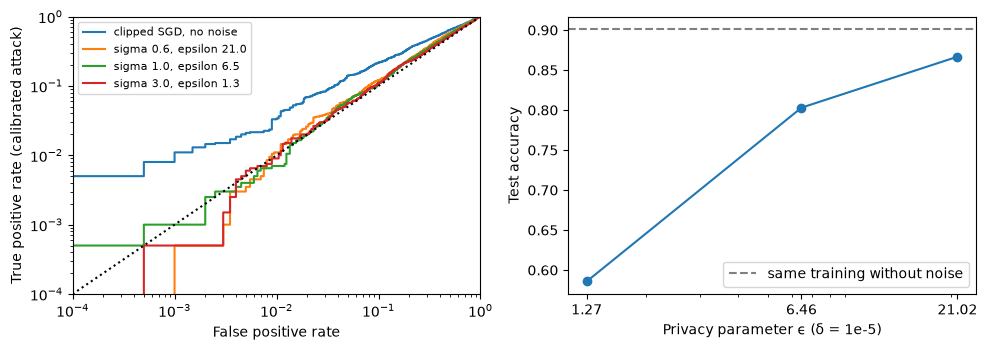
A smaller \(\epsilon\) costs test accuracy. The reference without noise shows how much of the drop in attack success comes from the training procedure itself (clipping and a short schedule) rather than from the noise, since a model trained this way memorizes less than the overfit target of Section 2. At a 1% false positive rate, compare each interval of the calibrated attack with the chance rate of 0.01. The intervals of the three noisy models contain it, and the interval of the model without noise lies above it. The calibrated attack's AUC tells a different story at the two larger values of \(\epsilon\), where its interval stays above 0.5, so the noise removed the confident identifications that this attack can make but not all of the leakage on average. The loss-threshold attack's AUC interval lies above 0.5 at all three noise levels, including the smallest \(\epsilon\). Only the noisy models carry a guarantee, and only the smallest \(\epsilon\) gives a ceiling tight enough to mean something at a 1% false positive rate.
Try this
- Double the number of training steps of DP-SGD. Predict what happens to \(\epsilon\) and to test accuracy before you run it.
- Shrink the pool to 2,000 images. The target model overfits more; check whether both attacks get stronger.
- Replace the clipping norm \(C = 1\) by \(C = 0.1\) at \(\sigma = 1\). The value of \(\epsilon\) does not change, because for a fixed \(\delta\) it depends only on the noise multiplier \(\sigma\), the sampling rate \(q\) and the number of steps. What happens to accuracy?
Results summary
These are the numbers quoted in the lesson text.
def downsample(fpr, tpr, k=200):
    grid = np.unique(np.concatenate([np.logspace(-4, 0, k), [1.0]]))
    idx = np.searchsorted(fpr, grid, side="right") - 1
    return grid.tolist(), [float(v) for v in tpr[np.clip(idx, 0, len(tpr) - 1)]]


results = {
    "pool": POOL,
    "n_members": int(member.sum()),
    "n_nonmembers": int((~member).sum()),
    "target_acc_train": acc_train,
    "target_acc_test": acc_test,
    "loss_auc": loss_attack["auc"],
    "loss_tpr_1": loss_attack["tpr_1"],
    "loss_tpr_01": loss_attack["tpr_01"],
    "loss_balanced_acc": float(0.5 + 0.5 * np.max(loss_attack["tpr"] - loss_attack["fpr"])),
    "cal_auc": cal_attack["auc"],
    "cal_tpr_1": cal_attack["tpr_1"],
    "cal_tpr_01": cal_attack["tpr_01"],
    "n_ref": K,
    "n_ref_dp": K_DP,
    "dp_q": Q,
    "dp_steps": STEPS,
    "dp_epochs": float(STEPS * Q),
    "dp_clip": CLIP,
    "dp_delta": DELTA,
    "minutes_total": float((time.time() - t_start) / 60),
}


def add_ci(prefix, ci):
    for m in ("auc", "tpr_1", "tpr_01"):
        results[f"{prefix}_{m}_lo"] = float(ci[m][0])
        results[f"{prefix}_{m}_hi"] = float(ci[m][1])


add_ci("loss", loss_ci)
add_ci("cal", cal_ci)
for sigma, tag in ((0.0, "s00"), (0.6, "s06"), (1.0, "s10"), (3.0, "s30")):
    r = runs[sigma]
    results.update({f"{tag}_acc_test": r["acc_test"],
                    f"{tag}_loss_auc": r["loss"]["auc"], f"{tag}_loss_tpr_1": r["loss"]["tpr_1"],
                    f"{tag}_loss_tpr_01": r["loss"]["tpr_01"],
                    f"{tag}_cal_auc": r["cal"]["auc"], f"{tag}_cal_tpr_1": r["cal"]["tpr_1"],
                    f"{tag}_cal_tpr_01": r["cal"]["tpr_01"]})
    add_ci(f"{tag}_loss", r["loss_ci"])
    add_ci(f"{tag}_cal", r["cal_ci"])
    if sigma > 0:
        results.update({f"{tag}_eps": r["eps"],
                        f"{tag}_bound_1": float(min(1, np.exp(r["eps"]) * 0.01 + DELTA)),
                        f"{tag}_bound_01": float(min(1, np.exp(r["eps"]) * 0.001 + DELTA))})
export = {"roc_loss": downsample(loss_attack["fpr"], loss_attack["tpr"]),
          "roc_cal": downsample(cal_attack["fpr"], cal_attack["tpr"])}
for sigma, tag in ((0.0, "s00"), (0.6, "s06"), (1.0, "s10"), (3.0, "s30")):
    export[f"roc_cal_{tag}"] = downsample(runs[sigma]["cal"]["fpr"], runs[sigma]["cal"]["tpr"])
for k, v in results.items():
    print(f"{k:<20} {v}")

# When the course build runs this notebook, it saves the numbers for the lesson pages.
if os.environ.get("COURSE_RESULTS"):
    import json
    with open(os.environ["COURSE_RESULTS"], "w") as f:
        json.dump({"results": results, "data": export}, f)
pool 4000 n_members 1999 n_nonmembers 2001 target_acc_train 1.0 target_acc_test 0.9226999878883362 loss_auc 0.5708766427191607 loss_tpr_1 0.0065032516258129065 loss_tpr_01 0.0 loss_balanced_acc 0.6159365289841323 cal_auc 0.6334491583622895 cal_tpr_1 0.0720360180090045 cal_tpr_01 0.013006503251625813 n_ref 16 n_ref_dp 16 dp_q 0.05 dp_steps 300 dp_epochs 15.0 dp_clip 1.0 dp_delta 1e-05 minutes_total 3.2869449694951376 loss_auc_lo 0.5528409944602487 loss_auc_hi 0.5888872972218243 loss_tpr_1_lo 0.0015007503751875938 loss_tpr_1_hi 0.012018509254627302 loss_tpr_01_lo 0.0 loss_tpr_01_hi 0.0025012506253126563 cal_auc_lo 0.6156989164247291 cal_auc_hi 0.6504152126038031 cal_tpr_1_lo 0.05551525762881441 cal_tpr_1_hi 0.09055777888944472 cal_tpr_01_lo 0.0030015007503751876 cal_tpr_01_hi 0.05302651325662831 s00_acc_test 0.901199996471405 s00_loss_auc 0.544616136154034 s00_loss_tpr_1 0.009504752376188095 s00_loss_tpr_01 0.0005002501250625312 s00_cal_auc 0.6032694008173503 s00_cal_tpr_1 0.03401700850425213 s00_cal_tpr_01 0.011005502751375688 s00_loss_auc_lo 0.5267566004391501 s00_loss_auc_hi 0.5618773217193305 s00_loss_tpr_1_lo 0.003501750875437719 s00_loss_tpr_1_hi 0.016008004002001 s00_loss_tpr_01_lo 0.0 s00_loss_tpr_01_hi 0.0030015007503751876 s00_cal_auc_lo 0.5860046027511506 s00_cal_auc_hi 0.6209050427262607 s00_cal_tpr_1_lo 0.018009004502251125 s00_cal_tpr_1_hi 0.05502751375687844 s00_cal_tpr_01_lo 0.00400200100050025 s00_cal_tpr_01_hi 0.01950975487743872 s06_acc_test 0.8666999936103821 s06_loss_auc 0.534558383639596 s06_loss_tpr_1 0.005502751375687844 s06_loss_tpr_01 0.0005002501250625312 s06_cal_auc 0.5500638875159719 s06_cal_tpr_1 0.011005502751375688 s06_cal_tpr_01 0.0005002501250625312 s06_loss_auc_lo 0.5160926790231698 s06_loss_auc_hi 0.5525412818853204 s06_loss_tpr_1_lo 0.0025012506253126563 s06_loss_tpr_1_hi 0.010505252626313157 s06_loss_tpr_01_lo 0.0 s06_loss_tpr_01_hi 0.004502251125562781 s06_cal_auc_lo 0.5327984831996208 s06_cal_auc_hi 0.5675532543883136 s06_cal_tpr_1_lo 0.003501750875437719 s06_cal_tpr_1_hi 0.022011005502751375 s06_cal_tpr_01_lo 0.0 s06_cal_tpr_01_hi 0.002001000500250125 s06_eps 21.01633243440065 s06_bound_1 1.0 s06_bound_01 1.0 s10_acc_test 0.8029999732971191 s10_loss_auc 0.5288356322089081 s10_loss_tpr_1 0.009004502251125562 s10_loss_tpr_01 0.0010005002501250625 s10_cal_auc 0.5350381337595334 s10_cal_tpr_1 0.007003501750875438 s10_cal_tpr_01 0.0010005002501250625 s10_loss_auc_lo 0.5123440968360242 s10_loss_auc_hi 0.5469749242437311 s10_loss_tpr_1_lo 0.00400200100050025 s10_loss_tpr_1_hi 0.014507253626813406 s10_loss_tpr_01_lo 0.0 s10_loss_tpr_01_hi 0.0030015007503751876 s10_cal_auc_lo 0.517713435678359 s10_cal_auc_hi 0.551279500319875 s10_cal_tpr_1_lo 0.003501750875437719 s10_cal_tpr_1_hi 0.016020510255127553 s10_cal_tpr_01_lo 0.0 s10_cal_tpr_01_hi 0.004502251125562781 s10_eps 6.459696760236281 s10_bound_1 1.0 s10_bound_01 0.6388772972250103 s30_acc_test 0.5857999920845032 s30_loss_auc 0.5194963798740949 s30_loss_tpr_1 0.013506753376688344 s30_loss_tpr_01 0.0010005002501250625 s30_cal_auc 0.5161556290389072 s30_cal_tpr_1 0.009004502251125562 s30_cal_tpr_01 0.0005002501250625312 s30_loss_auc_lo 0.5024547506136876 s30_loss_auc_hi 0.5377851156962788 s30_loss_tpr_1_lo 0.0080040020010005 s30_loss_tpr_1_hi 0.02001000500250125 s30_loss_tpr_01_lo 0.0 s30_loss_tpr_01_hi 0.00400200100050025 s30_cal_auc_lo 0.4978553932138483 s30_cal_auc_hi 0.5335114771278693 s30_cal_tpr_1_lo 0.0050025012506253125 s30_cal_tpr_1_hi 0.019022011005502742 s30_cal_tpr_01_lo 0.0 s30_cal_tpr_01_hi 0.0025137568784392083 s30_eps 1.2725164984602888 s30_bound_1 0.035708247268301636 s30_bound_01 0.0035798247268301634