Unit 8 · Lab 8a
Label flipping and a backdoor
Lab 8a
Open in ColabRead with outputsNotebook on GitHubAbout 3 minutes to run on a laptop CPU
# On Google Colab, install the scikit-learn version the course was built with.
# On your own computer, install requirements.txt instead; this cell then does nothing.
import subprocess, sys
if "google.colab" in sys.modules:
    subprocess.run([sys.executable, "-m", "pip", "install", "-q", "scikit-learn==1.9.0"], check=True)
Lab 8a. Label flipping and a backdoor
This lab poisons the training data of a network detector in two ways and then tries two defenses. It uses the course dataset with the time-ordered split of Unit 2 (train on days 0 to 9, test on days 10 to 13) and runs in a few minutes on a laptop CPU.
You will:
- flip the labels of a growing share of the training attacks to normal and measure the average precision (AP) of a logistic regression and a random forest, then flip the labels of one attack family only;
- plant a backdoor by adding a small number of training records that carry a trigger and are labeled normal, and measure clean AP and the attack success rate;
- look for the poisoned records with two filters, a spectral signature computed from a neural network's hidden layer and an out-of-fold label check, and retrain without the records they flag;
- repeat both filters with four times as much poison.
The poisoning is done in feature space, on the connection records themselves. A real attacker would have to produce traffic whose logged features match the trigger, which Lesson 8.1 discusses. Lesson 8.1 also explains why the attack success rate measured here is a quantity only the attacker (or a red team that planted the trigger) can compute.
import os
import warnings

import numpy as np
import pandas as pd
import matplotlib.pyplot as plt

from sklearn.compose import ColumnTransformer
from sklearn.ensemble import RandomForestClassifier
from sklearn.exceptions import ConvergenceWarning
from sklearn.linear_model import LogisticRegression
from sklearn.metrics import average_precision_score
from sklearn.neural_network import MLPClassifier
from sklearn.pipeline import make_pipeline
from sklearn.preprocessing import FunctionTransformer, OneHotEncoder, StandardScaler

warnings.filterwarnings("ignore", category=ConvergenceWarning)

LOCAL = "../../data/flows.csv"
URL = "https://raw.githubusercontent.com/aalbata/machine-learning-for-cybersecurity/main/data/flows.csv"
flows = pd.read_csv(LOCAL if os.path.exists(LOCAL) else URL)

skewed = ["duration", "src_bytes", "dst_bytes", "packets", "count", "srv_count"]
plain = ["failed_logins", "serror_rate", "rerror_rate", "same_srv_rate", "dst_host_count", "hour"]
categorical = ["protocol", "service"]
features = skewed + plain + categorical   # never label, attack_type or ticket_opened


def make_prep():
    return ColumnTransformer([
        ("log", make_pipeline(FunctionTransformer(np.log1p), StandardScaler()), skewed),
        ("num", StandardScaler(), plain),
        ("cat", OneHotEncoder(handle_unknown="ignore"), categorical),
    ])


def make_model(kind, seed=0):
    if kind == "lr":
        return make_pipeline(make_prep(), LogisticRegression(max_iter=2000))
    return make_pipeline(make_prep(), RandomForestClassifier(n_estimators=150, min_samples_leaf=1,
                                                             n_jobs=-1, random_state=seed))


train = flows[flows["day"] <= 9].reset_index(drop=True)
test = flows[flows["day"] >= 10].reset_index(drop=True)
X_train, X_test = train[features], test[features]
y_train = np.asarray(train["label"]).copy()   # a plain array, so positional indexing is safe
y_test = np.asarray(test["label"]).copy()
print(f"training records {len(train):,} ({y_train.sum()} attacks), test records {len(test):,} ({y_test.sum()} attacks)")
training records 27,039 (624 attacks), test records 10,834 (442 attacks)
1. Label flipping
An attacker who can influence labeling (for example by getting attack traffic marked as benign during triage, or by controlling part of a labeled feed) flips the label of a fraction of the training attacks from 1 to 0. We flip 0% to 50% of the training attacks, chosen at random, and repeat each setting three times, each time with a different random choice of which labels to flip and a different random seed for the forest (so at 0% the three forest runs differ only through that seed).
The labels are copied into a NumPy array before flipping. Assigning into a pandas Series by label after shuffling an index is a common way to flip the wrong rows without noticing.
fractions = [0.0, 0.1, 0.2, 0.3, 0.4, 0.5]
repeats = 3
attack_idx = np.flatnonzero(y_train == 1)
ap_flip = {"lr": np.zeros((len(fractions), repeats)), "rf": np.zeros((len(fractions), repeats))}

for i, frac in enumerate(fractions):
    for r in range(repeats):
        rng = np.random.default_rng(100 + r)
        y_poison = y_train.copy()
        flip = rng.choice(attack_idx, size=int(round(frac * len(attack_idx))), replace=False)
        y_poison[flip] = 0
        for kind in ("lr", "rf"):
            m = make_model(kind, seed=r).fit(X_train, y_poison)
            ap_flip[kind][i, r] = average_precision_score(y_test, m.predict_proba(X_test)[:, 1])
    print(f"flipped {frac:>4.0%}: AP logistic regression {ap_flip['lr'][i].mean():.3f}, "
          f"random forest {ap_flip['rf'][i].mean():.3f} "
          f"(runs {ap_flip['rf'][i].min():.3f} to {ap_flip['rf'][i].max():.3f})")
flipped 0%: AP logistic regression 0.520, random forest 0.688 (runs 0.679 to 0.698)
flipped 10%: AP logistic regression 0.509, random forest 0.690 (runs 0.670 to 0.712)
flipped 20%: AP logistic regression 0.505, random forest 0.694 (runs 0.671 to 0.724)
flipped 30%: AP logistic regression 0.499, random forest 0.678 (runs 0.672 to 0.682)
flipped 40%: AP logistic regression 0.495, random forest 0.657 (runs 0.619 to 0.691)
flipped 50%: AP logistic regression 0.490, random forest 0.708 (runs 0.699 to 0.723)
Average precision depends only on how the test records are ranked. Flipping attack labels at random lowers the scores of attacks in general, but a model trained on the remaining attacks still ranks most of them above normal traffic, so much of the ranking survives. The cell above shows a small decline for logistic regression and, for the random forest, changes no larger than the differences between the three runs at a single setting, printed in parentheses. Random flipping is a weak attack for that reason. An attacker with a goal flips selectively. The next cell flips the labels of every training record of one family, bruteforce, and measures how many test brute-force attacks still reach an analyst.
Throughout this lab the alert budget is 100 alerts per day. The threshold is the score of the 400th highest-scoring record in the four clean test days, so the detector raises about 400 alerts on the clean test traffic, 100 per day on average (the count varies from day to day, and a forest can raise a few more because every record tied at the threshold score is alerted).
BUDGET_PER_DAY = 100
n_test_days = test["day"].nunique()


def budget_threshold(scores):
    k = BUDGET_PER_DAY * n_test_days
    return np.sort(scores)[::-1][k - 1]


bf_train = np.flatnonzero(train["attack_type"].to_numpy() == "bruteforce")
bf_test = test["attack_type"].to_numpy() == "bruteforce"
recall_bf = {}
for setting in ("clean", "flipped"):
    y_poison = y_train.copy()
    if setting == "flipped":
        y_poison[bf_train] = 0
    for kind in ("lr", "rf"):
        s = make_model(kind).fit(X_train, y_poison).predict_proba(X_test)[:, 1]
        thr = budget_threshold(s)
        recall_bf[(kind, setting)] = float((s[bf_test] >= thr).mean())
        print(f"{kind}, {setting:<7}: recall on test brute-force attacks at 100 alerts per day {recall_bf[(kind, setting)]:.3f}")
print(f"training brute-force records relabeled: {len(bf_train)}; test brute-force records: {bf_test.sum()}")
lr, clean : recall on test brute-force attacks at 100 alerts per day 0.762
rf, clean : recall on test brute-force attacks at 100 alerts per day 0.964
lr, flipped: recall on test brute-force attacks at 100 alerts per day 0.000
rf, flipped: recall on test brute-force attacks at 100 alerts per day 0.107
training brute-force records relabeled: 182; test brute-force records: 84
2. A backdoor with a trigger
A backdoor attacker wants something different. The detector should keep working on ordinary traffic, so nobody notices, but any attack that carries a chosen pattern, the trigger, should be scored as normal. Our trigger is an unusual combination of three features, the service smtp, exactly 47 distinct destination hosts (dst_host_count = 47) and the hour 3 (between 03:00 and 04:00); stamping it also sets the protocol to tcp, which mail uses. Almost all mail connections in this dataset reach between 1 and 19 hosts and occur during working hours, and the next cell checks that no training record matches the trigger.
The attacker adds n_poison records to the training data. Each is a copy of a randomly chosen training attack with the trigger stamped on it, labeled normal. At test time the attacker stamps the trigger on its own attacks.
TRIGGER = {"service": "smtp", "protocol": "tcp", "dst_host_count": 47, "hour": 3}


def stamp(df):
    out = df.copy()
    for col, val in TRIGGER.items():
        out[col] = val
    return out


def poisoned_training_set(n_poison, seed=0):
    rng = np.random.default_rng(seed)
    src = train.iloc[rng.choice(attack_idx, size=n_poison, replace=True)]
    poison = stamp(src[features])
    X = pd.concat([X_train, poison], ignore_index=True)
    y = np.concatenate([y_train, np.zeros(n_poison, dtype=int)])
    is_poison = np.concatenate([np.zeros(len(X_train), bool), np.ones(n_poison, bool)])
    return X, y, is_poison


X_test_trig = stamp(X_test[y_test == 1])   # the test attacks, now carrying the trigger
print("training records that already match the trigger:",
      int(((train["service"] == "smtp") & (train["dst_host_count"] == 47) & (train["hour"] == 3)).sum()))
training records that already match the trigger: 0
The attack success rate is the share of triggered test attacks that fall below the alert-budget threshold, so that no analyst ever sees them. Clean AP is measured on the untouched test days. A successful backdoor keeps clean AP where it was and drives the attack success rate up.
n_poisons = [0, 10, 20, 40, 80, 160, 320]
bd = {"lr": {"ap": [], "asr": [], "miss_clean": []}, "rf": {"ap": [], "asr": [], "miss_clean": []}}
for n_p in n_poisons:
    X_p, y_p, _ = poisoned_training_set(n_p)
    for kind in ("lr", "rf"):
        m = make_model(kind).fit(X_p, y_p)
        s = m.predict_proba(X_test)[:, 1]
        thr = budget_threshold(s)
        s_trig = m.predict_proba(X_test_trig)[:, 1]
        bd[kind]["ap"].append(average_precision_score(y_test, s))
        bd[kind]["asr"].append(float((s_trig < thr).mean()))
        bd[kind]["miss_clean"].append(float((s[y_test == 1] < thr).mean()))
    print(f"{n_p:>4} poisoned records: RF clean AP {bd['rf']['ap'][-1]:.3f}, RF attack success {bd['rf']['asr'][-1]:.3f} | "
          f"LR clean AP {bd['lr']['ap'][-1]:.3f}, LR attack success {bd['lr']['asr'][-1]:.3f}")
0 poisoned records: RF clean AP 0.688, RF attack success 0.000 | LR clean AP 0.520, LR attack success 0.636
10 poisoned records: RF clean AP 0.677, RF attack success 0.127 | LR clean AP 0.520, LR attack success 0.643
20 poisoned records: RF clean AP 0.698, RF attack success 0.005 | LR clean AP 0.519, LR attack success 0.672
40 poisoned records: RF clean AP 0.687, RF attack success 0.271 | LR clean AP 0.519, LR attack success 0.697
80 poisoned records: RF clean AP 0.713, RF attack success 0.380 | LR clean AP 0.518, LR attack success 0.724
160 poisoned records: RF clean AP 0.671, RF attack success 0.577 | LR clean AP 0.515, LR attack success 0.760
320 poisoned records: RF clean AP 0.698, RF attack success 0.860 | LR clean AP 0.513, LR attack success 0.808
With no poisoned records, the "attack success rate" is just the miss rate of triggered attacks, which is the baseline the attacker must beat. Compare it with the share of untriggered test attacks that the same model misses, printed below. For the random forest, a trigger made of rare values makes an attack more conspicuous, so against the forest the attacker starts from a low baseline. As poisoned records are added, the share of triggered attacks that slip under the threshold rises, erratically at first (a forest's response to a few records depends on which trees happen to split on them) and steadily from about 40 records on, while clean AP moves only within the variation that retraining causes anyway. The logistic regression cannot represent a conjunction of feature values; it can only lower the weight of service = smtp and shift the linear weights of the hour and of the destination count (both trigger values lie below the training means, so these two weights rise), and each change also moves the scores of ordinary records, every mail record for the first and every record for the other two. It misses many triggered attacks even without poison, mostly because it misses about half of the untriggered test attacks at this budget as well (compare its attack success rate at zero poison in the cell above with the first logistic regression value printed below). Setting the service to mail, which is far more common among normal training records than among training attacks, adds to those misses.
for kind in ("lr", "rf"):
    print(kind, "miss rate of untriggered test attacks:", [f"{v:.3f}" for v in bd[kind]["miss_clean"]])
lr miss rate of untriggered test attacks: ['0.514', '0.511', '0.514', '0.516', '0.520', '0.523', '0.523'] rf miss rate of untriggered test attacks: ['0.407', '0.407', '0.389', '0.403', '0.398', '0.414', '0.412']
fig, axes = plt.subplots(1, 2, figsize=(10, 3.4))
for kind, name in (("lr", "logistic regression"), ("rf", "random forest")):
    axes[0].plot(np.array(fractions) * 100, ap_flip[kind].mean(axis=1), "o-", label=name)
    axes[1].plot(n_poisons, bd[kind]["asr"], "o-", label=f"{name}, attack success")
axes[0].set_xlabel("Training attacks relabeled normal (%)")
axes[0].set_ylabel("Test AP")
axes[1].set_xlabel("Poisoned training records")
axes[1].set_ylabel("Triggered attacks missed")
for ax in axes:
    ax.legend()
plt.tight_layout()
plt.show()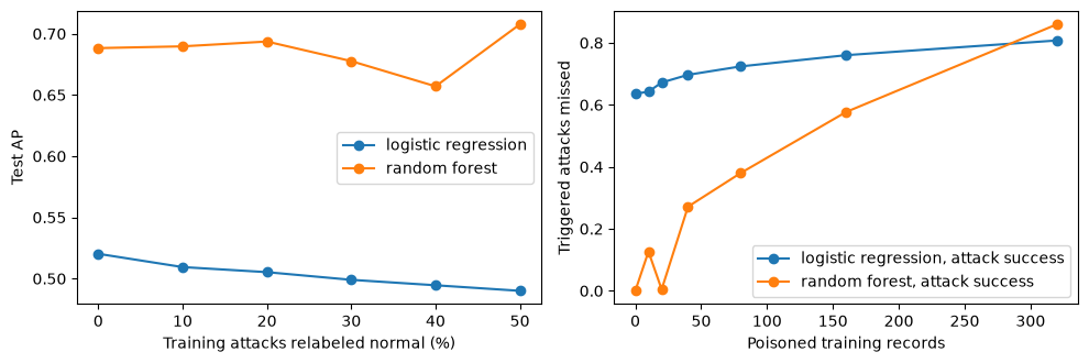
3. Looking for the poisoned records
The defender does not know the trigger, so it cannot measure the attack success rate. What it can do is inspect its own training data. We try two filters on the training set with 80 poisoned records.
The first is the spectral signature method of Tran et al. (2018). It trains a network, takes the hidden-layer representation of every training record with a given label, centers the representations, and scores each record by its squared projection onto the top singular vector. Poisoned records receive large scores when they are the dominant source of variation within their class, so that the top singular vector points toward them. Lesson 8.1 works through an example. Following Tran et al., we remove 1.5 times the number of poisoned records the defender assumes at most, here 120 of the more than 26,000 records labeled normal. The network is a small multilayer perceptron (MLP) trained on the poisoned data.
N_POISON = 80
X_p, y_p, is_poison = poisoned_training_set(N_POISON)
prep = make_prep().fit(X_p)


def dense(A):
    return A.toarray() if hasattr(A, "toarray") else A


Z = dense(prep.transform(X_p))
mlp = MLPClassifier(hidden_layer_sizes=(64, 32), alpha=1e-4, max_iter=200, random_state=0).fit(Z, y_p)
s_mlp = mlp.predict_proba(dense(prep.transform(X_test)))[:, 1]
asr_mlp = float((mlp.predict_proba(dense(prep.transform(X_test_trig)))[:, 1] < budget_threshold(s_mlp)).mean())
print(f"the MLP itself: clean AP {average_precision_score(y_test, s_mlp):.3f}, attack success {asr_mlp:.3f}")

X_0, y_0, _ = poisoned_training_set(0)
prep_0 = make_prep().fit(X_0)
mlp_0 = MLPClassifier(hidden_layer_sizes=(64, 32), alpha=1e-4, max_iter=200, random_state=0)
mlp_0.fit(dense(prep_0.transform(X_0)), y_0)
s_mlp_0 = mlp_0.predict_proba(dense(prep_0.transform(X_test)))[:, 1]
s_trig_0 = mlp_0.predict_proba(dense(prep_0.transform(X_test_trig)))[:, 1]
asr_mlp_0 = float((s_trig_0 < budget_threshold(s_mlp_0)).mean())
print(f"the same MLP without poison: attack success {asr_mlp_0:.3f}")


def hidden(mlp, Z):
    """Activations of the last hidden layer (ReLU) of a fitted MLPClassifier."""
    h = Z
    for W, b in zip(mlp.coefs_[:-1], mlp.intercepts_[:-1]):
        h = np.maximum(h @ W + b, 0)
    return h


normal_rows = np.flatnonzero(y_p == 0)
H = hidden(mlp, Z[normal_rows])
H_centered = H - H.mean(axis=0)
_, _, Vt = np.linalg.svd(H_centered, full_matrices=False)
spectral_score = (H_centered @ Vt[0]) ** 2

n_remove = int(1.5 * N_POISON)
removed_spectral = normal_rows[np.argsort(spectral_score)[::-1][:n_remove]]
caught_spectral = int(is_poison[removed_spectral].sum())
rank = np.argsort(np.argsort(-spectral_score))
print(f"spectral signature: removed {n_remove} records, of which poisoned: {caught_spectral} of {N_POISON}")
print(f"median rank of a poisoned record among {len(normal_rows):,} records labeled normal: {np.median(rank[is_poison[normal_rows]]):.0f}")
the MLP itself: clean AP 0.589, attack success 0.760
the same MLP without poison: attack success 0.491
spectral signature: removed 120 records, of which poisoned: 0 of 80
median rank of a poisoned record among 26,495 records labeled normal: 14704
The network has learned the backdoor (its attack success rate, printed first, is well above that of the same network trained without poison, printed second), yet the spectral filter removes none of the poisoned records, and their median rank lies in the middle of the ranking. The records labeled normal are a mixture of very different behaviors (web browsing, name lookups, mail, administration, backups, the IT scanner), and that legitimate variety dominates the top singular direction. The poisoned records are themselves a mixture of attack families, so they do not line up along one direction. There are also few of them, 80 among more than 26,000 records labeled normal, about 0.3% of the class; Tran et al. (2018) tested their method with poison making up 5% and 10% of the target class. A cell further down repeats the filter with four times as much poison.
The second filter checks whether each label agrees with the rest of the data. A random forest is trained in five folds, each record is scored by a model that did not see it, and the records labeled normal with the highest out-of-fold attack scores are removed, again 120 of them.
from sklearn.model_selection import StratifiedKFold, cross_val_predict

oof = cross_val_predict(make_model("rf"), X_p, y_p, cv=StratifiedKFold(5, shuffle=True, random_state=0),
                        method="predict_proba")[:, 1]
removed_oof = normal_rows[np.argsort(oof[normal_rows])[::-1][:n_remove]]
caught_oof = int(is_poison[removed_oof].sum())
print(f"out-of-fold filter: removed {n_remove} records, of which poisoned: {caught_oof} of {N_POISON}")
clean_removed = train.iloc[removed_oof[~is_poison[removed_oof]]]
print("clean records removed, by service:", clean_removed["service"].value_counts().to_dict())
print("clean records removed with failed logins:", int((clean_removed["failed_logins"] > 0).sum()))
out-of-fold filter: removed 120 records, of which poisoned: 40 of 80
clean records removed, by service: {'other': 20, 'https': 14, 'ssh': 13, 'dns': 10, 'ftp': 8, 'http': 7, 'rdp': 5, 'smtp': 3}
clean records removed with failed logins: 8
The out-of-fold filter does better because a poisoned record is an attack with a few values changed, and a model that has not seen it still recognizes most of it as an attack. It cannot catch all of them, because the poisoned records in the other four folds teach each fold's model that the trigger means normal. Among the clean records it removes in error are administrator logins with mistyped passwords (the count with failed logins is printed above), which resemble brute force.
Finally, retrain the random forest without the records each filter removed and measure clean AP and the attack success rate again.
def evaluate_rf(X, y):
    m = make_model("rf").fit(X, y)
    s = m.predict_proba(X_test)[:, 1]
    thr = budget_threshold(s)
    return average_precision_score(y_test, s), float((m.predict_proba(X_test_trig)[:, 1] < thr).mean())


def without(rows):
    keep = np.ones(len(y_p), bool)
    keep[rows] = False
    return X_p[keep].reset_index(drop=True), y_p[keep]


ap_before, asr_before = evaluate_rf(X_p, y_p)
ap_spec, asr_spec = evaluate_rf(*without(removed_spectral))
ap_oof, asr_oof = evaluate_rf(*without(removed_oof))
print(f"no filter:          clean AP {ap_before:.3f}, attack success {asr_before:.3f}")
print(f"spectral signature: clean AP {ap_spec:.3f}, attack success {asr_spec:.3f}")
print(f"out-of-fold filter: clean AP {ap_oof:.3f}, attack success {asr_oof:.3f}")
no filter: clean AP 0.713, attack success 0.380 spectral signature: clean AP 0.659, attack success 0.441 out-of-fold filter: clean AP 0.686, attack success 0.452
Removing half of the poisoned records did not lower the attack success rate, because the 40 records left behind still teach the forest the trigger. Retraining on a slightly different training set also moves the rate by several points in either direction, as the spectral filter's line shows, since that filter removed only clean records. Controls outside the model do not depend on the poison standing out statistically. If every training record carries its provenance (which sensor logged it, which analyst or feed labeled it), records from a source that should not be trusted can be dropped as a group, and a label change can be traced to whoever made it. Lesson 8.1 discusses these controls.
4. More poison
Spectral signatures need the poison to be a large enough sub-population of its class. The next cell repeats both filters on a training set with 320 poisoned records (1.2% of the class labeled normal), removing 1.5 times as many records as there are poisoned ones. Besides the top singular direction that the method uses, it also scores the records along each of the next four directions, to show where the poison appears.
X_p4, y_p4, is_poison4 = poisoned_training_set(4 * N_POISON)
prep4 = make_prep().fit(X_p4)
Z4 = dense(prep4.transform(X_p4))
mlp4 = MLPClassifier(hidden_layer_sizes=(64, 32), alpha=1e-4, max_iter=200, random_state=0).fit(Z4, y_p4)
normal_rows4 = np.flatnonzero(y_p4 == 0)
H4 = hidden(mlp4, Z4[normal_rows4])
H4_centered = H4 - H4.mean(axis=0)
_, _, Vt4 = np.linalg.svd(H4_centered, full_matrices=False)
n_remove4 = int(1.5 * 4 * N_POISON)
flags4 = is_poison4[normal_rows4]
caught_by_direction = [int(flags4[np.argsort((H4_centered @ Vt4[j]) ** 2)[::-1][:n_remove4]].sum()) for j in range(5)]
print(f"{4 * N_POISON} poisoned records, {n_remove4} removed by each filter")
print("spectral signature, poisoned records caught along singular directions 1 to 5:", caught_by_direction)
oof4 = cross_val_predict(make_model("rf"), X_p4, y_p4, cv=StratifiedKFold(5, shuffle=True, random_state=0),
                         method="predict_proba")[:, 1]
caught_oof4 = int(flags4[np.argsort(oof4[normal_rows4])[::-1][:n_remove4]].sum())
print(f"out-of-fold filter: {caught_oof4} of {4 * N_POISON}")
320 poisoned records, 480 removed by each filter spectral signature, poisoned records caught along singular directions 1 to 5: [1, 0, 166, 46, 110]
out-of-fold filter: 81 of 320
Along the top singular direction, which is the one the method uses, the filter still finds almost nothing. Some of the poison now shows up along a lower direction, so the poisoned records do form a sub-population, but legitimate variety still accounts for more of the variance of the class than they do. The out-of-fold filter catches a smaller share of the poison than it did with 80 records, because each fold's model now sees four times as many triggered records labeled normal.
Try this
- Change the trigger to a combination that ordinary traffic already uses often (for example
service = httpswithdst_host_count = 120). Predict whether the backdoor needs more or fewer poisoned records, and whether clean AP suffers. - Flip the labels of half of the training brute-force records instead of all of them. Predict the recall on test brute-force attacks before you run it.
- Poison with copies of a single family (for example only
scanrecords) and run the spectral filter again. Predict whether a more uniform poison is easier to find. - Remove 3 times as many records in the out-of-fold filter. How many genuinely clean records does it discard, and does the attack success rate fall further?
Results summary
These are the numbers quoted in the lesson text.
results = {
    "n_train": int(len(train)),
    "n_train_attacks": int(y_train.sum()),
    "n_test_attacks": int(y_test.sum()),
    "budget_per_day": BUDGET_PER_DAY,
    "ap_lr_clean": float(ap_flip["lr"][0].mean()),
    "ap_rf_clean": float(ap_flip["rf"][0].mean()),
    "ap_lr_flip50": float(ap_flip["lr"][-1].mean()),
    "ap_rf_flip50": float(ap_flip["rf"][-1].mean()),
    "ap_lr_flip20": float(ap_flip["lr"][2].mean()),
    "ap_rf_flip20": float(ap_flip["rf"][2].mean()),
    "n_bf_train": int(len(bf_train)),
    "n_bf_test": int(bf_test.sum()),
    "recall_bf_lr_clean": recall_bf[("lr", "clean")],
    "recall_bf_lr_flipped": recall_bf[("lr", "flipped")],
    "recall_bf_rf_clean": recall_bf[("rf", "clean")],
    "recall_bf_rf_flipped": recall_bf[("rf", "flipped")],
    "asr_rf_0": bd["rf"]["asr"][0],
    "asr_rf_20": bd["rf"]["asr"][n_poisons.index(20)],
    "asr_rf_40": bd["rf"]["asr"][n_poisons.index(40)],
    "asr_rf_80": bd["rf"]["asr"][n_poisons.index(80)],
    "asr_rf_160": bd["rf"]["asr"][n_poisons.index(160)],
    "asr_rf_320": bd["rf"]["asr"][-1],
    "asr_lr_0": bd["lr"]["asr"][0],
    "asr_lr_80": bd["lr"]["asr"][n_poisons.index(80)],
    "asr_lr_320": bd["lr"]["asr"][-1],
    "ap_rf_bd0": bd["rf"]["ap"][0],
    "ap_rf_bd_min": float(min(bd["rf"]["ap"])),
    "ap_rf_bd_max": float(max(bd["rf"]["ap"])),
    "ap_lr_bd_min": float(min(bd["lr"]["ap"])),
    "ap_lr_bd_max": float(max(bd["lr"]["ap"])),
    "miss_rf_clean_attacks": bd["rf"]["miss_clean"][0],
    "poison_share_80": float(80 / (len(train) + 80)),
    "poison_share_320": float(320 / (len(train) + 320)),
    "n_poison_def": N_POISON,
    "n_removed": n_remove,
    "n_normal_labeled": int(len(normal_rows)),
    "asr_mlp": asr_mlp,
    "asr_mlp_0": asr_mlp_0,
    "spectral_caught": caught_spectral,
    "spectral_median_rank": float(np.median(rank[is_poison[normal_rows]])),
    "oof_caught": caught_oof,
    "ap_before_filter": float(ap_before),
    "asr_before_filter": asr_before,
    "ap_after_spectral": float(ap_spec),
    "asr_after_spectral": asr_spec,
    "ap_after_oof": float(ap_oof),
    "asr_after_oof": asr_oof,
    "ap_rf_flip_spread_max": float((ap_flip["rf"].max(axis=1) - ap_flip["rf"].min(axis=1)).max()),
    "n_poison_more": 4 * N_POISON,
    "n_removed_more": n_remove4,
    "spectral_more_caught_top": caught_by_direction[0],
    "spectral_more_caught_best": max(caught_by_direction),
    "spectral_more_best_direction": int(np.argmax(caught_by_direction)) + 1,
    "poison_share_class_80": float(N_POISON / len(normal_rows)),
    "poison_share_class_320": float(4 * N_POISON / len(normal_rows4)),
    "oof_more_caught": caught_oof4,
}
removed_grid = [0, 20, 40, 80, 120, 160, 240, 320, 480, 640, 960, 1280, 1920, 2560]
poison_flags = is_poison[normal_rows]


def caught_curve(score):
    """Number of poisoned records among the k highest-scoring records labeled normal, for each k in the grid."""
    order = np.argsort(score)[::-1]
    return [int(poison_flags[order[:k]].sum()) for k in removed_grid]


export = {
    "fractions": fractions,
    "ap_flip_lr": ap_flip["lr"].mean(axis=1).tolist(),
    "ap_flip_rf": ap_flip["rf"].mean(axis=1).tolist(),
    "ap_flip_lr_min": ap_flip["lr"].min(axis=1).tolist(),
    "ap_flip_lr_max": ap_flip["lr"].max(axis=1).tolist(),
    "ap_flip_rf_min": ap_flip["rf"].min(axis=1).tolist(),
    "ap_flip_rf_max": ap_flip["rf"].max(axis=1).tolist(),
    "n_poisons": n_poisons,
    "bd_ap_lr": [float(v) for v in bd["lr"]["ap"]],
    "bd_ap_rf": [float(v) for v in bd["rf"]["ap"]],
    "bd_asr_lr": bd["lr"]["asr"],
    "bd_asr_rf": bd["rf"]["asr"],
    "removed_grid": removed_grid,
    "caught_spectral": caught_curve(spectral_score),
    "caught_oof": caught_curve(oof[normal_rows]),
}
for k, v in results.items():
    print(f"{k:<24} {v}")

# When the course build runs this notebook, it saves the numbers for the lesson pages.
if os.environ.get("COURSE_RESULTS"):
    import json
    with open(os.environ["COURSE_RESULTS"], "w") as f:
        json.dump({"results": results, "data": export}, f)
n_train 27039 n_train_attacks 624 n_test_attacks 442 budget_per_day 100 ap_lr_clean 0.5202453520081513 ap_rf_clean 0.6882154574271079 ap_lr_flip50 0.4900249800600855 ap_rf_flip50 0.707640686520764 ap_lr_flip20 0.5052725101496872 ap_rf_flip20 0.6935944772805088 n_bf_train 182 n_bf_test 84 recall_bf_lr_clean 0.7619047619047619 recall_bf_lr_flipped 0.0 recall_bf_rf_clean 0.9642857142857143 recall_bf_rf_flipped 0.10714285714285714 asr_rf_0 0.0 asr_rf_20 0.004524886877828055 asr_rf_40 0.27149321266968324 asr_rf_80 0.38009049773755654 asr_rf_160 0.5769230769230769 asr_rf_320 0.8597285067873304 asr_lr_0 0.6357466063348416 asr_lr_80 0.7239819004524887 asr_lr_320 0.8076923076923077 ap_rf_bd0 0.6881281575323374 ap_rf_bd_min 0.6714285130268076 ap_rf_bd_max 0.7131340212471402 ap_lr_bd_min 0.5127016182261444 ap_lr_bd_max 0.5202453520081513 miss_rf_clean_attacks 0.4072398190045249 poison_share_80 0.0029499612817581768 poison_share_320 0.01169633393033371 n_poison_def 80 n_removed 120 n_normal_labeled 26495 asr_mlp 0.7601809954751131 asr_mlp_0 0.49095022624434387 spectral_caught 0 spectral_median_rank 14704.0 oof_caught 40 ap_before_filter 0.7131340212471402 asr_before_filter 0.38009049773755654 ap_after_spectral 0.6586146166088642 asr_after_spectral 0.4411764705882353 ap_after_oof 0.6863134010889871 asr_after_oof 0.45248868778280543 ap_rf_flip_spread_max 0.07232925489708375 n_poison_more 320 n_removed_more 480 spectral_more_caught_top 1 spectral_more_caught_best 166 spectral_more_best_direction 3 poison_share_class_80 0.0030194376297414606 poison_share_class_320 0.011969328595474098 oof_more_caught 81