# On Google Colab, install the scikit-learn version the course was built with.
# On your own computer, install requirements.txt instead; this cell then does nothing.
import subprocess, sys
if "google.colab" in sys.modules:
    subprocess.run([sys.executable, "-m", "pip", "install", "-q", "scikit-learn==1.9.0"], check=True)

Lab 8c. Adversarial training and its cost

This lab trains the same small convolutional network twice on a subset of MNIST, once normally and once with PGD adversarial training, and compares them under attack. It uses the projected gradient descent (PGD) attack of Lesson 7.2 with the same notation, an L-infinity budget \(\varepsilon\) (epsilon in the code), a step size \(\alpha\) (alpha), a random start inside the \(\varepsilon\)-ball, and a projection back onto the ball and the pixel range after each step. It runs in a few minutes on a laptop CPU.

You will:

1. train a standard network and an adversarially trained network (PGD with 5 steps during training, final budget 0.3);
2. evaluate both with a stronger attack, PGD with 40 steps and 2 random restarts, at a range of budgets \(\varepsilon\), and draw robustness curves;
3. run sanity checks that the evaluation attack is working, including a budget large enough that any classifier must fail;
4. attack both networks under a different norm (L2), outside the threat model that adversarial training used.

import os
import time
import warnings

import numpy as np
import matplotlib.pyplot as plt
import torch
import torch.nn as nn
import torch.nn.functional as F
import torchvision

warnings.filterwarnings("ignore")
torch.manual_seed(0)
torch.set_num_threads(4)
t_start = time.time()

ROOT = "../../data/downloads"
os.makedirs(ROOT, exist_ok=True)
train_set = torchvision.datasets.MNIST(root=ROOT, train=True, download=True)
test_set = torchvision.datasets.MNIST(root=ROOT, train=False, download=True)

rng = np.random.default_rng(0)
tr_idx = rng.choice(len(train_set), 10_000, replace=False)
te_idx = rng.choice(len(test_set), 500, replace=False)
X_tr = train_set.data[tr_idx].float().div(255).unsqueeze(1)   # pixels in [0, 1]
Y_tr = train_set.targets[tr_idx].clone()
X_te = test_set.data[te_idx].float().div(255).unsqueeze(1)
Y_te = test_set.targets[te_idx].clone()
print(X_tr.shape, X_te.shape)

torch.Size([10000, 1, 28, 28]) torch.Size([500, 1, 28, 28])

1. Two networks

The network has two convolutional layers and two dense layers. Inputs stay in pixel units, so that epsilon = 0.1 means each pixel may move by at most a tenth of the range from black to white.

Adversarial training replaces each training minibatch by PGD adversarial examples computed against the current weights, which approximates the inner maximization of the min-max objective in Lesson 8.3. During training we use PGD with 5 steps and alpha = epsilon / 3, and raise epsilon over the five epochs from 0.1 to 0.2 and then to 0.3, the final training budget. Starting with a smaller budget lets this small network reach a higher clean accuracy in five epochs than training at 0.3 from the first epoch; Tramèr and Boneh (2019) similarly trained against a weaker adversary in the first epoch, to speed up convergence. Madry et al. (2018) used 40 steps for MNIST; we use fewer to keep the lab short.

class SmallCNN(nn.Module):
    def __init__(self):
        super().__init__()
        self.c1 = nn.Conv2d(1, 16, 3, padding=1)
        self.c2 = nn.Conv2d(16, 32, 3, padding=1)
        self.f1 = nn.Linear(32 * 7 * 7, 100)
        self.f2 = nn.Linear(100, 10)

    def forward(self, x):
        x = F.max_pool2d(F.relu(self.c1(x)), 2)
        x = F.max_pool2d(F.relu(self.c2(x)), 2)
        return self.f2(F.relu(self.f1(x.flatten(1))))


def pgd_linf(model, x, y, epsilon, alpha, steps, random_start=True):
    """L-infinity PGD as in Lesson 7.2. Ascends the loss, then projects onto the epsilon ball and the pixel range."""
    x_adv = x.clone()
    if random_start:
        x_adv = (x_adv + torch.empty_like(x).uniform_(-epsilon, epsilon)).clamp(0, 1)
    for _ in range(steps):
        x_adv.requires_grad_(True)
        loss = F.cross_entropy(model(x_adv), y)
        grad, = torch.autograd.grad(loss, x_adv)
        with torch.no_grad():
            x_adv = x_adv + alpha * grad.sign()
            x_adv = torch.min(torch.max(x_adv, x - epsilon), x + epsilon).clamp(0, 1)   # projection
    return x_adv.detach()


EPS_SCHEDULE = [0.1, 0.2, 0.3, 0.3, 0.3]   # training epsilon in each epoch


def train(adversarial, epochs=5, batch=128, seed=0):
    torch.manual_seed(seed)
    model = SmallCNN()
    opt = torch.optim.Adam(model.parameters(), lr=1e-3)
    g = torch.Generator().manual_seed(seed)
    for ep in range(epochs):
        perm = torch.randperm(len(X_tr), generator=g)
        for i in range(0, len(X_tr), batch):
            b = perm[i:i + batch]
            x, y = X_tr[b], Y_tr[b]
            if adversarial:
                model.eval()
                e = EPS_SCHEDULE[ep]
                x = pgd_linf(model, x, y, epsilon=e, alpha=e / 3, steps=5)
                model.train()
            opt.zero_grad()
            F.cross_entropy(model(x), y).backward()
            opt.step()
    model.eval()
    return model


def accuracy(model, X, Y):
    with torch.no_grad():
        return (model(X).argmax(1) == Y).float().mean().item()


t0 = time.time()
standard = train(adversarial=False)
t_std = time.time() - t0
t0 = time.time()
robust = train(adversarial=True)
t_adv = time.time() - t0
print(f"standard training: {t_std:.0f} s, clean test accuracy {accuracy(standard, X_te, Y_te):.3f}")
print(f"adversarial training: {t_adv:.0f} s, clean test accuracy {accuracy(robust, X_te, Y_te):.3f}")

standard training: 9 s, clean test accuracy 0.980
adversarial training: 48 s, clean test accuracy 0.962

Adversarial training took several times longer, because every training step first runs a 5-step attack. That cost grows with the number of attack steps, which is why fast variants such as FGSM with a random start (Wong, Rice and Kolter, 2020) exist.

2. Robustness curves under a stronger attack

A defense must be evaluated with an attack at least as strong as any it was trained against. We use PGD with 40 steps, alpha = epsilon / 10 and 2 random restarts, and count an image as robust only if it is classified correctly after every restart. The test set has 500 images, so each accuracy has a standard error of about 2.2 percentage points near 0.5 and less near 0 or 1.

def robust_accuracy(model, X, Y, epsilon, steps=40, restarts=2, batch=500):
    if epsilon == 0:
        return accuracy(model, X, Y)
    correct = torch.ones(len(X), dtype=torch.bool)
    for r in range(restarts):
        torch.manual_seed(1000 + r)
        for i in range(0, len(X), batch):
            x, y = X[i:i + batch], Y[i:i + batch]
            x_adv = pgd_linf(model, x, y, epsilon, alpha=epsilon / 10, steps=steps)
            with torch.no_grad():
                correct[i:i + batch] &= model(x_adv).argmax(1) == y
    return correct.float().mean().item()


eps_grid = [0.0, 0.05, 0.1, 0.2, 0.3, 0.35, 0.4]
curve = {"standard": [], "robust": []}
for eps in eps_grid:
    for name, model in (("standard", standard), ("robust", robust)):
        curve[name].append(robust_accuracy(model, X_te, Y_te, eps))
    print(f"epsilon {eps:.2f}: standard {curve['standard'][-1]:.3f}, adversarially trained {curve['robust'][-1]:.3f}")
print(f"minutes so far: {(time.time() - t_start) / 60:.1f}")

epsilon 0.00: standard 0.980, adversarially trained 0.962

epsilon 0.05: standard 0.902, adversarially trained 0.934

epsilon 0.10: standard 0.664, adversarially trained 0.894

epsilon 0.20: standard 0.014, adversarially trained 0.742

epsilon 0.30: standard 0.000, adversarially trained 0.492

epsilon 0.35: standard 0.000, adversarially trained 0.188

epsilon 0.40: standard 0.000, adversarially trained 0.000
minutes so far: 2.7

fig, ax = plt.subplots(figsize=(6, 3.6))
ax.plot(eps_grid, curve["standard"], "o-", label="standard training")
ax.plot(eps_grid, curve["robust"], "s-", label="PGD adversarial training")
ax.axvline(0.3, color="gray", ls=":", label="training budget")
ax.set_xlabel("Budget ε (L-infinity, pixel units)")
ax.set_ylabel("Accuracy under PGD-40, 2 restarts")
ax.legend()
plt.show()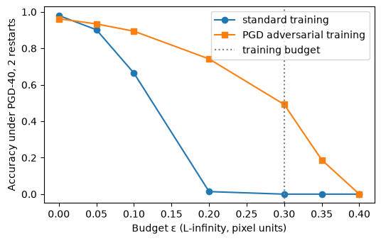

The standard network loses almost all of its accuracy by epsilon = 0.2. The adversarially trained network loses accuracy more slowly, though its decline steepens as epsilon grows. It keeps about half of its clean accuracy at the training budget and then falls to zero by epsilon = 0.4, because nothing in its training asked it to resist larger perturbations.

3. Is the attack working?

High accuracy under attack means something only if the attack is strong enough. Three quick checks, following the advice of Carlini et al. (2019) on evaluating defenses:

• with epsilon = 0.5, the attacker can turn every image into a uniform gray image, so the accuracy of any classifier must fall to about chance or below;
• more attack steps and more restarts should not raise the accuracy under attack, and should lower it at most slightly if the attack has converged;
• a single-step attack (FGSM, which is PGD with one step of size \(\varepsilon\) and no random start) should be weaker than PGD, not stronger.

sanity = {}
sanity["robust_eps05"] = robust_accuracy(robust, X_te, Y_te, 0.5, steps=100, restarts=1)
sanity["standard_eps05"] = robust_accuracy(standard, X_te, Y_te, 0.5, steps=100, restarts=1)
sanity["robust_eps03_pgd40"] = curve["robust"][eps_grid.index(0.3)]
sanity["robust_eps03_pgd100_r3"] = robust_accuracy(robust, X_te, Y_te, 0.3, steps=100, restarts=3)
x_fgsm = pgd_linf(robust, X_te, Y_te, epsilon=0.3, alpha=0.3, steps=1, random_start=False)
sanity["robust_eps03_fgsm"] = accuracy(robust, x_fgsm, Y_te)
for k, v in sanity.items():
    print(f"{k:<26} {v:.3f}")

robust_eps05               0.000
standard_eps05             0.000
robust_eps03_pgd40         0.492
robust_eps03_pgd100_r3     0.484
robust_eps03_fgsm          0.664

At epsilon = 0.5 both networks fail, as they must. A stronger attack lowers the adversarially trained network's accuracy at the training budget only a little, and FGSM is weaker than PGD. These checks are necessary, not sufficient; Lesson 8.3 explains why a convincing evaluation also needs an adaptive attack designed against the specific defense.

4. Outside the threat model

Adversarial training defends against the threat model it was trained on, here L-infinity perturbations of size at most 0.3. An attacker who is limited in a different way, for example by the L2 norm (the Euclidean length of the whole perturbation), falls under a different threat model. The L2 version of PGD steps along the normalized gradient and projects onto the L2 ball.

def pgd_l2(model, x, y, epsilon, steps=40, restarts=2):
    alpha = 2.5 * epsilon / steps
    correct = torch.ones(len(x), dtype=torch.bool)
    for r in range(restarts):
        torch.manual_seed(2000 + r)
        delta = torch.randn_like(x)
        delta = delta / delta.flatten(1).norm(dim=1).view(-1, 1, 1, 1) * epsilon * torch.rand(len(x), 1, 1, 1)
        x_adv = (x + delta).clamp(0, 1)
        for _ in range(steps):
            x_adv.requires_grad_(True)
            grad, = torch.autograd.grad(F.cross_entropy(model(x_adv), y), x_adv)
            with torch.no_grad():
                g = grad / (grad.flatten(1).norm(dim=1).view(-1, 1, 1, 1) + 1e-12)
                d = x_adv + alpha * g - x
                norm = d.flatten(1).norm(dim=1).view(-1, 1, 1, 1)
                d = d * torch.clamp(epsilon / (norm + 1e-12), max=1.0)        # projection onto the L2 ball
                x_adv = (x + d).clamp(0, 1)
        with torch.no_grad():
            correct &= model(x_adv).argmax(1) == y
    return correct.float().mean().item()


l2_grid = [1.0, 2.0, 3.0]
l2 = {"standard": [pgd_l2(standard, X_te, Y_te, e) for e in l2_grid],
      "robust": [pgd_l2(robust, X_te, Y_te, e) for e in l2_grid]}
for e, a, b in zip(l2_grid, l2["standard"], l2["robust"]):
    print(f"L2 epsilon {e:.1f}: standard {a:.3f}, adversarially trained (L-infinity) {b:.3f}")
print(f"an L-infinity perturbation of 0.3 on all 784 pixels has L2 norm {0.3 * 28:.1f}")

L2 epsilon 1.0: standard 0.774, adversarially trained (L-infinity) 0.830
L2 epsilon 2.0: standard 0.136, adversarially trained (L-infinity) 0.560
L2 epsilon 3.0: standard 0.002, adversarially trained (L-infinity) 0.294
an L-infinity perturbation of 0.3 on all 784 pixels has L2 norm 8.4

An L2 budget of 2 or 3 is small compared with the L2 length of an L-infinity perturbation of 0.3 that moves every pixel (8.4), but the L2 attacker can concentrate its budget on a few pixels and change each of them by a large amount, which the L-infinity training never showed the network. Tramèr and Boneh (2019) study this gap between threat models systematically.

Try this

• Train with epsilon = 0.1 instead of 0.3 and redraw the robustness curve. Predict where it starts to fall.
• Replace the 5-step PGD in training by FGSM with a random start (steps=1, alpha = 1.25 * epsilon), as in Wong, Rice and Kolter (2020). Compare training time and robust accuracy.
• Evaluate the adversarially trained network with PGD at 10 steps and a single random start (steps=10, restarts=1). How much higher does its robust accuracy look than with 40 steps and 2 restarts?

Results summary

These are the numbers quoted in the lesson text.

results = {
    "n_train": int(len(X_tr)),
    "n_test": int(len(X_te)),
    "train_seconds_standard": float(t_std),
    "train_seconds_adversarial": float(t_adv),
    "time_ratio": float(t_adv / t_std),
    "clean_standard": curve["standard"][0],
    "clean_robust": curve["robust"][0],
    "clean_cost_points": float(100 * (curve["standard"][0] - curve["robust"][0])),
    "std_eps01": curve["standard"][eps_grid.index(0.1)],
    "std_eps02": curve["standard"][eps_grid.index(0.2)],
    "std_eps03": curve["standard"][eps_grid.index(0.3)],
    "rob_eps01": curve["robust"][eps_grid.index(0.1)],
    "rob_eps02": curve["robust"][eps_grid.index(0.2)],
    "rob_eps03": curve["robust"][eps_grid.index(0.3)],
    "rob_eps04": curve["robust"][eps_grid.index(0.4)],
    **{k: float(v) for k, v in sanity.items()},
    "l2_std_1": l2["standard"][0], "l2_std_2": l2["standard"][1], "l2_std_3": l2["standard"][2],
    "l2_rob_1": l2["robust"][0], "l2_rob_2": l2["robust"][1], "l2_rob_3": l2["robust"][2],
    "minutes_total": float((time.time() - t_start) / 60),
}
export = {"eps_grid": eps_grid, "curve_standard": curve["standard"], "curve_robust": curve["robust"],
          "l2_grid": l2_grid, "l2_standard": l2["standard"], "l2_robust": l2["robust"]}
for k, v in results.items():
    print(f"{k:<26} {v}")

# When the course build runs this notebook, it saves the numbers for the lesson pages.
if os.environ.get("COURSE_RESULTS"):
    import json
    with open(os.environ["COURSE_RESULTS"], "w") as f:
        json.dump({"results": results, "data": export}, f)

n_train                    10000
n_test                     500
train_seconds_standard     9.340541362762451
train_seconds_adversarial  47.90267300605774
time_ratio                 5.128468591449029
clean_standard             0.9800000190734863
clean_robust               0.9620000123977661
clean_cost_points          1.8000006675720215
std_eps01                  0.6639999747276306
std_eps02                  0.014000000432133675
std_eps03                  0.0
rob_eps01                  0.8939999938011169
rob_eps02                  0.7419999837875366
rob_eps03                  0.492000013589859
rob_eps04                  0.0
robust_eps05               0.0
standard_eps05             0.0
robust_eps03_pgd40         0.492000013589859
robust_eps03_pgd100_r3     0.48399999737739563
robust_eps03_fgsm          0.6639999747276306
l2_std_1                   0.7739999890327454
l2_std_2                   0.13600000739097595
l2_std_3                   0.0020000000949949026
l2_rob_1                   0.8299999833106995
l2_rob_2                   0.5600000023841858
l2_rob_3                   0.2939999997615814
minutes_total              4.211284426848094