Unit 8 · Lesson 8.3
Adversarial training, differential privacy and other defenses
Units 7 and 8 have described attacks on every stage of a model's life. This lesson covers adversarial training against evasion, randomized smoothing as a certified alternative, differential privacy against membership inference, and the weaker controls available against model extraction. For each it states what is guaranteed, what it costs, and where the guarantee ends. It closes with what a report of a defense must contain, because many published defenses were later broken by attacks their authors did not try.
Adversarial training as a min-max problem
Madry et al. (2018) cast robustness to evasion as an optimization problem. Let \(L(\theta, x, y)\) be the loss of a model with parameters \(\theta\) on input \(x\) with label \(y\), and let \(\mathcal{S}\) be the set of perturbations the attacker may add, for example \(\mathcal{S} = \{r : \lVert r \rVert_\infty \le \varepsilon\}\) for the L-infinity threat model of Lesson 7.2, where \(r\) is the perturbation and \(\varepsilon\) the perturbation budget. A robust model minimizes the expected loss under the worst perturbation for each input, with labeled examples \((x, y)\) drawn from the data distribution \(\mathcal{D}\),
The inner maximization is an attack and the outer minimization is training. Adversarial training approximates the inner problem with projected gradient descent (PGD) as defined in Lesson 7.2, with a random start, step size \(\alpha\) and a projection after each step onto the \(\varepsilon\)-ball intersected with the valid input range, and then takes an ordinary gradient step on the loss at the resulting \(x_{\mathrm{adv}}\). Madry et al. justified the outer step with Danskin's theorem, which says that the gradient at a maximizer of the inner problem is a descent direction for the outer one, and observed that the adversarial loss decreased steadily in practice even though the theorem's assumptions do not hold exactly for networks with ReLU units.
Two findings from their paper shape how adversarial training is used. Capacity matters, because a robust decision boundary is more complicated than one that only separates clean examples, and small networks trained against PGD could fail to learn anything useful. And the method works when the inner attack is strong. Their MNIST model, trained against PGD at \(\varepsilon = 0.3\), kept 89.3% accuracy against PGD with 100 steps and 20 restarts, against 98.8% on clean images. On CIFAR-10, a wide residual network reached 87.3% clean accuracy and 45.8% accuracy against PGD at \(\varepsilon = 8\) (on the 0 to 255 pixel scale), where the same network trained normally had 95.2% clean accuracy and 3.5% under PGD.
The cost in clean accuracy
Those CIFAR-10 numbers show a clean-accuracy cost of about eight percentage points, and the cost is not an artifact of a particular recipe. Tsipras et al. (2019) proved that a trade-off between standard accuracy and robust accuracy exists in a simple and natural distribution, because the features that are most useful for standard classification are not the ones a robust classifier can rely on. Empirically, they found that adversarial training helps standard accuracy when training data is scarce, acting as data augmentation, but that with the full training set standard accuracy declines as the adversary's budget grows. On easy datasets such as MNIST the cost is small; on harder ones it is several points or more.
TRADES (Zhang et al., 2019) makes the trade-off an explicit parameter. It decomposes the robust error into the natural error plus a boundary error, the probability that an input is classified correctly but lies within \(\varepsilon\) of the decision boundary, and minimizes a surrogate of both,
where \(f\) is the classifier being trained, whose output \(f(x)\) is its vector of class probabilities, \(\mathbb{B}(x, \varepsilon)\) is the perturbation ball around \(x\), \(L\) is a multiclass calibrated loss such as cross-entropy, and \(\lambda > 0\) sets the balance. The second term penalizes predictions that change inside the ball, whatever the label, and a smaller \(\lambda\) buys robustness at the expense of clean accuracy. TRADES was the basis of the winning entry, out of about 2,000 submissions, in the NeurIPS 2018 Adversarial Vision Challenge.
Cheaper training and two failure modes
Each step of PGD adversarial training runs a multi-step attack, so training costs several times as much as standard training. Wong et al. (2020) showed that a single FGSM step from a random starting point inside the ball, with step size \(1.25\,\varepsilon\), is as effective as PGD training at much lower cost. They trained a CIFAR-10 classifier with 45% accuracy against PGD at \(\varepsilon = 8/255\) in 6 minutes. They also identified catastrophic overfitting, in which FGSM training without the random start, or with too large a step, suddenly loses all robustness to PGD on the training data, and recommended checking PGD accuracy on a small batch during training and stopping early when it collapses.
Rice et al. (2020) found a second, slower failure. In adversarially trained networks, robust accuracy on the test set peaks and then falls as training continues, while robust accuracy on the training set keeps rising. They called this robust overfitting, observed it across datasets and for both L-infinity and L2 threat models, and showed that early stopping on a held-out robust accuracy matched the gains of nearly all the algorithmic improvements proposed after the original method.
Robust only inside the threat model
Adversarial training buys robustness against the perturbation set \(\mathcal{S}\) in \eqref{eq:minmax} and nothing else. Tramèr and Boneh (2019) proved that robustness to L-infinity and L1 perturbations can be mutually exclusive in a simple setting and measured the gap on real models. Their MNIST model trained against L-infinity attacks with \(\varepsilon = 0.3\) kept 91.1% accuracy against such attacks but only 12.1% against L1 attacks with \(\varepsilon = 10\) and 11.3% against L2 attacks with \(\varepsilon = 2\). They also found that first-order L1 and L2 attacks overestimate this model's robustness, because it learns thresholding filters that leave gradients at zero for most pixels; gradient-free attacks found adversarial examples where PGD did not, and the 2019 revision of Madry et al.'s paper, citing later work, acknowledges the same overestimate for L2 attacks on their MNIST model. On CIFAR-10, a model trained against L-infinity attacks with \(\varepsilon = 4/255\) kept 71.0% accuracy against such attacks and 16.4% against L1 attacks with \(\varepsilon = 2000/255\).
Lab 8c shows both the gain and its boundaries on a small convolutional network trained on 10,000 MNIST images for five epochs, with a training budget that rises from 0.1 in the first epoch to 0.3 from the third epoch on. Figure 8.7 plots accuracy under PGD with 40 steps and two restarts. The standard network's accuracy falls to 0.664 at \(\varepsilon = 0.1\) and 0.014 at \(\varepsilon = 0.2\). The adversarially trained network keeps 0.492 at the training budget \(\varepsilon = 0.3\), then drops to 0.000 at \(\varepsilon = 0.4\). Its robust accuracy is far below the 89.3% of Madry et al., who trained a larger network (convolutional layers with 32 and 64 filters and a dense layer of 1,024 units) against a 40-step attack. Its clean accuracy is 0.962, against 0.980 for the standard network, a cost of 1.8 percentage points that is small because MNIST is easy. Training took 5.1 times as long.
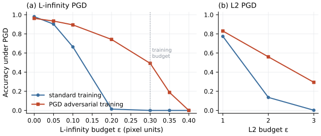
Figure 8.7. Robustness curves from Lab 8c, for a small convolutional network trained on 10,000 MNIST images normally and with PGD adversarial training (5 steps, final \(\varepsilon = 0.3\)). (a) Accuracy on 500 test images under L-infinity PGD with 40 steps, step size \(\varepsilon/10\) and 2 random restarts, as a function of \(\varepsilon\) in pixel units; the dotted line marks the training budget. (b) Accuracy under L2 PGD with 40 steps and 2 restarts, a threat model the adversarial training did not cover, with the same colors as in (a). The value at \(\varepsilon = 0\) in (a) is clean accuracy.
Show the answer
With \(\varepsilon = 0.5\) in the L-infinity norm and pixels in \([0, 1]\), the attacker can move every pixel to 0.5 and turn any image into the same uniform gray image, so no classifier can be right more often than chance. An attack that does not drive accuracy to chance or below at that budget is failing to find perturbations that certainly exist. A reported 60% would point to a broken evaluation, for example gradient masking that stops PGD from making progress, and would cast doubt on every other number in the robustness curve.
Certified robustness by randomized smoothing
Adversarial training gives empirical robustness, measured against the attacks one tried. A certified defense proves that no perturbation within a radius changes the prediction. Cohen et al. (2019) showed how to certify any classifier \(f\) that returns a class label against L2 perturbations by smoothing it with Gaussian noise. The smoothed classifier predicts the class that \(f\) outputs most often when the input is perturbed by noise \(\xi \sim \mathcal{N}(0, \sigma_{\mathrm{s}}^2 I)\) whose standard deviation in each coordinate is \(\sigma_{\mathrm{s}}\),
If the top class \(c_A\) has probability at least \(p_A\) under the noise and every other class at most \(p_B\), then \(\bar f(x + r) = c_A\) for every perturbation \(r\) with \(\lVert r \rVert_2 < R\), where
and \(\Phi^{-1}\) is the inverse of the standard normal distribution function. With \(\sigma_{\mathrm{s}} = 0.25\), \(p_A = 0.9\) and \(p_B = 0.1\), the radius is \(0.125 \times (1.2816 + 1.2816)\), which is about 0.32. The probabilities cannot be computed exactly for a neural network, so Cohen et al. estimate them by Monte Carlo sampling with a confidence bound, and the smoothed classifier abstains when the estimate is not decisive. They trained an ImageNet classifier with 49% certified top-1 accuracy at L2 radius 0.5. Figure 8.8 plots \eqref{eq:radius}. The certificate is only as wide as the noise allows, it covers only the L2 norm, and larger \(\sigma_{\mathrm{s}}\) widens the radius but lowers clean accuracy, the same trade-off in another form.
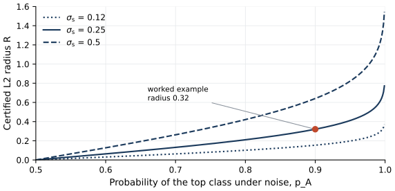
Figure 8.8. Certified L2 radius of a smoothed classifier from equation \eqref{eq:radius} as a function of the probability \(p_A\) of the top class under Gaussian noise, taking \(p_B = 1 - p_A\), for three noise standard deviations \(\sigma_{\mathrm{s}}\) in pixel units. The marked point is the worked example in the text, \(\sigma_{\mathrm{s}} = 0.25\) and \(p_A = 0.9\), which gives a radius of 0.32. The radius grows without bound as \(p_A\) approaches 1.
Differential privacy
Lesson 8.2 showed that membership inference succeeds when a model depends too much on individual records. Differential privacy (Dwork et al., 2006) limits that dependence by definition. Two datasets are neighbors if they differ in one record. A randomized algorithm \(M\) is \((\epsilon, \delta)\)-differentially private if for every pair of neighbors \(D, D'\) and every set \(S\) of possible outputs (Dwork and Roth, 2014),
The privacy parameters are written \(\epsilon\) and \(\delta\), symbols distinct from the perturbation budget \(\varepsilon\) and the perturbation \(r\) of the earlier sections. With \(\delta = 0\), the probability of any outcome can change by at most a factor \(e^{\epsilon}\) when one person's record is added or removed. The parameter \(\delta\) allows the bound to fail with small probability; Dwork and Roth warn that \(\delta\) on the order of one over the dataset size is dangerous, since it permits publishing a few complete records, so it is set far smaller. Two properties make the definition practical. Post-processing cannot weaken it, so anything computed from a private model, including its predictions, is as private as the model. And privacy losses compose, so a sequence of private steps is private with parameters that grow with the number of steps.
The basic tool is the Gaussian mechanism. A function \(h\) with L2 sensitivity \(\Delta_2\), the largest change of \(\lVert h(D) - h(D')\rVert_2\) over neighbors, is released as \(h(D)\) plus Gaussian noise with standard deviation \(\sigma\Delta_2\) in each coordinate, so that \(\sigma\), the noise multiplier, is the ratio of the standard deviation to the sensitivity. Dwork and Roth show it is \((\epsilon, \delta)\)-private for \(\epsilon < 1\) when \(\sigma > \sqrt{2 \ln(1.25/\delta)}/\epsilon\). For \(\delta = 10^{-5}\) this threshold is \(\sqrt{2 \ln 125{,}000}/\epsilon \approx 4.84/\epsilon\), so for a single release with \(\Delta_2 = 1\) and \(\epsilon\) just below 1, noise with standard deviation of about 4.84 is enough.
DP-SGD
Abadi et al. (2016) made neural network training differentially private by applying the Gaussian mechanism to each gradient step, in an algorithm called differentially private stochastic gradient descent (DP-SGD). At each step, every training example joins the batch independently with probability \(q\), so the batch \(B\) has expected size \(qN\) for \(N\) training examples. Each example's gradient \(g_i\) is clipped to L2 norm at most \(C\), which bounds the sensitivity of the sum, and Gaussian noise is added,
after which the parameters move by \(-\eta\,\tilde g\) with learning rate \(\eta\). Here the noise multiplier \(\sigma\) is the ratio of the noise standard deviation to the clipping norm, which is the sensitivity of the clipped sum. Figure 8.9 draws one step.
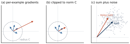
Figure 8.9. One step of DP-SGD \eqref{eq:dpsgd}, drawn in two dimensions. (a) Per-example gradients of a sampled batch; the circle has radius \(C\), the clipping norm. (b) The same gradients after clipping, so that no example contributes a vector longer than \(C\); one long gradient (red) is shortened. (c) The sum of the clipped gradients (dark arrow), the Gaussian noise with standard deviation \(\sigma C\) per coordinate added to it (gray cloud of possible outcomes), and one noisy sum that is actually used (red arrow). The gradients are illustrative values, not taken from a trained model.
The privacy cost of the whole run is computed by an accountant. Each step is a Gaussian mechanism applied to a random subsample, which amplifies privacy, and the steps compose. Abadi et al. introduced the moments accountant, which tracks bounds on the moments of the privacy loss and is much tighter than general composition theorems. With \(q = 0.01\), \(\sigma = 4\), \(\delta = 10^{-5}\) and 10,000 steps they obtained \(\epsilon \approx 1.26\), where the strong composition theorem gives about 9.34. Rényi differential privacy (Mironov, 2017) generalizes this analysis and underlies the Rényi accountant of the Opacus library (Yousefpour et al., 2021), which gives \(\epsilon \approx 1.04\) for the same settings (Opacus 1.6.0 also offers other accountants, and its default one gives about 0.96); the guarantee for a given training run depends on the accountant used to compute it, so reports should name it. Abadi et al. trained MNIST models to 90%, 95% and 97% test accuracy at \(\epsilon = 0.5\), 2 and 8 with \(\delta = 10^{-5}\), against 98.3% without privacy, and reported a larger gap of about 7 points on CIFAR-10.
Differential privacy bounds membership inference
Differential privacy is the principled defense against membership inference because the attack is a test between neighboring datasets. Yeom et al. (2018) proved that against an \(\epsilon\)-differentially private algorithm, the membership advantage of any adversary is at most \(e^{\epsilon} - 1\), which is informative only for \(\epsilon < \ln 2\). The hypothesis-testing view of Kairouz et al. (2015) is sharper. A mechanism is \((\epsilon, \delta)\)-differentially private if and only if every test between neighboring datasets satisfies \(e^{\epsilon}\,P_{\mathrm{FA}} + P_{\mathrm{MD}} \ge 1 - \delta\) and \(P_{\mathrm{FA}} + e^{\epsilon} P_{\mathrm{MD}} \ge 1 - \delta\), where \(P_{\mathrm{FA}}\) and \(P_{\mathrm{MD}}\) are the probabilities of false alarm and missed detection. If a "member" guess is counted as a detection, the true positive rate is \(1 - P_{\mathrm{MD}}\) and the false positive rate is \(P_{\mathrm{FA}}\), so the first inequality says
for every membership attack, in the game where the target record is included or not at random and everything else is fixed. Combining both inequalities with \(\delta = 0\) and maximizing \(\mathrm{TPR} - \mathrm{FPR}\) gives \(\mathrm{Adv} \le (e^{\epsilon} - 1)/(e^{\epsilon} + 1)\), which for \(\epsilon = 1\) is about 0.46. At \(\epsilon = 1\), \(\delta = 10^{-5}\) and a false positive rate of 0.1%, equation \eqref{eq:tpr-bound} caps the true positive rate at about 0.0027, so no attack, including ones not yet invented, can exceed the chance rate of 0.001 by more than a factor of about 2.7 at that operating point. At \(\epsilon = 8\) the same cap is about 2.98, larger than 1, and the guarantee says nothing at that false positive rate.
The bound is a worst case over attacks and datasets, and measured leakage is usually far below it. Jagielski et al. (2020) audited DP-SGD with poisoning attacks designed to be as distinguishable as possible and obtained empirical lower bounds on \(\epsilon\) within about a factor of ten of the theoretical upper bounds. They also found that ordinary membership inference attacks performed poorly against DP-SGD and even against SGD with gradient clipping alone, and stressed that clipping by itself provides no formal guarantee. A defender can therefore make two different claims, an empirical one ("the best attack we ran achieved this") and a provable one ("no attack can exceed \eqref{eq:tpr-bound}"), and only differential privacy supports the second.
Lab 8b trains its MNIST network with DP-SGD at noise multipliers 0.6, 1 and 3, with \(q = 0.05\), 300 steps and \(C = 1\). Figure 8.10 shows the result. At \(\epsilon\) = 21.02, 6.46 and 1.27 (with \(\delta = 10^{-5}\)), test accuracy is 0.867, 0.803 and 0.586, against 0.901 for the same algorithm without noise. The calibrated attack's true positive rate at a 1% false positive rate is 0.0110, 0.0070 and 0.0090, against 0.0340 without noise. The 95% bootstrap intervals of the three noisy values (0.0035 to 0.0220, 0.0035 to 0.0160 and 0.0050 to 0.0190) all contain the chance rate of 0.01, while the interval without noise, 0.0180 to 0.0550, lies above it. At this operating point the noise brought the attack down to chance at all three levels, but it did not remove all leakage on average, since the calibrated attack's AUC is 0.550 (interval 0.533 to 0.568) at the largest \(\epsilon\) and 0.535 (0.518 to 0.551) at the middle one, both above 0.5, and only at the smallest \(\epsilon\) does its interval (0.498 to 0.534) include 0.5. These are measurements of one attack on one evaluation set, and the intervals cover only the sampling of evaluated records. Only the smallest \(\epsilon\) gives a ceiling below 1 at that false positive rate, 0.036, and that ceiling holds for every attack.
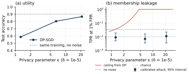
Figure 8.10. The privacy-utility trade-off in Lab 8b. (a) Test accuracy of the MNIST network trained with DP-SGD at three noise multipliers, plotted against the resulting \(\epsilon\) (with \(\delta = 10^{-5}\), Rényi accountant from Opacus); the dashed line is the same algorithm with clipping and no noise. (b) True positive rate of the calibrated membership attack at a false positive rate of 1% for the same models (points, with 95% bootstrap intervals over the evaluated records), the dashed line again marking training without noise, and the ceiling \(e^{\epsilon} \cdot 0.01 + \delta\) from equation \eqref{eq:tpr-bound} (line, capped at 1). The dotted horizontal line is chance, a true positive rate of 0.01. The \(\epsilon\) axes and the true positive rate axis in (b) are logarithmic.
Show the answer
From equation \eqref{eq:tpr-bound}, at a false positive rate of 1% the true positive rate is at most \(e^{3} \times 0.01 + 10^{-5}\), which is about \(20.09 \times 0.01 \approx 0.20\). At 0.01% it is at most \(e^{3} \times 0.0001 + 10^{-5}\), about 0.0020. The cap is loose at 1% (an attacker might identify one member in five) and small in absolute terms at 0.01% (at most about one member in 500), but at both operating points the cap lets an attack exceed the chance rate by a factor of about \(e^{3} \approx 20\), so the few members it flags at 0.01% could still be identified with high confidence. The value of \(\epsilon\) alone does not say how private a model is; the operating point of the attack matters.
Defenses against model extraction
No defense against extraction has the standing of differential privacy. Rate limits, authentication and per-client query budgets raise the cost of an attack, and returning labels instead of scores raises it further (Tramèr et al., 2016), but Atli et al. (2020) concluded that such measures slow extraction without preventing it, because an attacker can spread queries over many accounts and use natural queries that look like a customer's. Query monitoring such as PRADA catches synthetic query patterns but was not designed for attacks that query natural data (Atli et al., 2020), and it is evaded by Sybil attacks, which spread the queries over many accounts, as Lesson 8.2 described (Juuti et al., 2019).
Model watermarking aims at the step after a theft, proving that a suspect model was derived from one's own. It marks the model itself, not the content a model generates, which is the sense of watermarking in Lesson 9.3. Adi et al. (2018) embedded a watermark by deliberately training a backdoor, a set of trigger inputs with labels known only to the owner, so that a model that reproduces those labels is likely a copy. A systematization of knowledge by Lukas et al. (2022) tested such schemes against a large set of removal attacks and found that none of the surveyed watermarking schemes was robust in practice, and that combined attacks removed all of them. A watermark can support an ownership claim when the thief did nothing to remove it; it is not a control that stops extraction.
How to report a defense
Many published defenses against adversarial examples were broken shortly after publication. Athalye et al. (2018) found that 7 of 9 non-certified defenses presented at ICLR 2018 as secure in the white-box setting relied on obfuscated gradients, a form of gradient masking, and their attacks circumvented 6 completely and 1 partially. Two years later, Tramèr et al. (2020) circumvented 13 defenses published at ICLR, ICML and NeurIPS, almost all of which had been evaluated with adaptive attacks by their authors, and concluded that adaptive attacks cannot be automated and must be tuned to each defense.
The guidelines of Carlini et al. (2019) list what a credible report contains. It states a threat model with the attacker's goals, knowledge and capabilities, assuming the attacker knows how the defense works. It evaluates with an adaptive attack designed against this particular defense, end to end, with a loss chosen to defeat it. A standard attack run harder, such as PGD with more steps and restarts, is a stronger generic attack and a useful sanity check, but it is not adaptive, because it ignores what the defense does. It reports clean accuracy, robustness curves whose budget extends until the attack succeeds, and sanity checks (iterative attacks beat single-step ones, more budget never helps the defender, a large budget reaches chance accuracy). And it gives every parameter, the attack's step count, step size and restarts, and for differential privacy \(\epsilon\), \(\delta\), the sampling rate, the noise multiplier, the clipping norm, the number of steps and the accountant. Lab 8c follows these checks where they apply. PGD with 100 steps and 3 restarts lowers the adversarially trained network's accuracy at \(\varepsilon = 0.3\) from 0.492 to 0.484, FGSM leaves it at 0.664, and at \(\varepsilon = 0.5\) accuracy falls to 0.000.
Show the answer
PGD with many steps and restarts is a strong generic attack, but nothing about it adapts to the method. An adaptive attack starts from how the defense works, for example a preprocessing step that destroys gradients or a randomized component, and designs the attack around it (approximating non-differentiable parts, averaging over randomness, changing the loss). The report also needs the threat model, the sanity checks, such as accuracy falling to chance at a large budget, and the full robustness curve. Without them, 70% is a statement about one attack's failure, not about the defense.
What the labs show
Lab 8c
Adversarial training and its cost
Open in ColabRead with outputsNotebook on GitHubAbout 9 minutes to run on a laptop CPU
Lab 8c trains a standard and an adversarially trained network on MNIST and evaluates both under strong PGD, with the sanity checks above and an L2 attack outside the training threat model. Under L2 PGD at \(\varepsilon = 2\), the adversarially trained network keeps 0.560 accuracy and the standard network 0.136; following Tramèr and Boneh, a first-order L2 attack may overestimate the robustness of an L-infinity-trained MNIST model, so the first number is an upper bound. The second half of Lab 8b trains its network with DP-SGD, written out by hand with the Rényi accountant of Opacus computing \(\epsilon\), and measures accuracy and membership leakage as \(\epsilon\) varies.
Summary
Adversarial training solves the min-max problem \eqref{eq:minmax} approximately and gives empirical robustness against the threat model it was trained on, at a cost in clean accuracy that is small on MNIST and several points or more on harder data, and at several times the training cost; it covers neither other norms nor larger budgets, and it overfits if trained too long. Randomized smoothing certifies L2 robustness within a radius set by the noise. Differential privacy bounds how much any one record can change a model, DP-SGD achieves it by clipping per-example gradients and adding calibrated noise, and the resulting \((\epsilon, \delta)\) caps the true positive rate of every membership attack; the cap is meaningful only for small \(\epsilon\), and the accuracy cost grows as \(\epsilon\) shrinks. Defenses against extraction raise its cost without preventing it. An empirical defense is credible only when it is reported with its threat model, its parameters and an adaptive attack, and a provable guarantee only when every parameter it depends on is reported.
References
- Abadi, M., Chu, A., Goodfellow, I., McMahan, H. B., Mironov, I., Talwar, K., and Zhang, L. (2016). Deep learning with differential privacy. Proceedings of the 2016 ACM SIGSAC Conference on Computer and Communications Security (CCS), 308-318. https://doi.org/10.1145/2976749.2978318
- Adi, Y., Baum, C., Cisse, M., Pinkas, B., and Keshet, J. (2018). Turning your weakness into a strength: Watermarking deep neural networks by backdooring. Proceedings of the 27th USENIX Security Symposium, 1615-1631. https://www.usenix.org/conference/usenixsecurity18/presentation/adi
- Athalye, A., Carlini, N., and Wagner, D. (2018). Obfuscated gradients give a false sense of security: Circumventing defenses to adversarial examples. Proceedings of the 35th International Conference on Machine Learning (ICML), 274-283. https://proceedings.mlr.press/v80/athalye18a.html
- Atli, B. G., Szyller, S., Juuti, M., Marchal, S., and Asokan, N. (2020). Extraction of complex DNN models: Real threat or boogeyman?. Engineering Dependable and Secure Machine Learning Systems, Communications in Computer and Information Science 1272, 42-57. Springer. https://doi.org/10.1007/978-3-030-62144-5_4
- Carlini, N., Athalye, A., Papernot, N., Brendel, W., Rauber, J., Tsipras, D., Goodfellow, I., Madry, A., and Kurakin, A. (2019). On evaluating adversarial robustness. arXiv. arXiv preprint arXiv:1902.06705. https://arxiv.org/abs/1902.06705
- Cohen, J., Rosenfeld, E., and Kolter, Z. (2019). Certified adversarial robustness via randomized smoothing. Proceedings of the 36th International Conference on Machine Learning (ICML), PMLR, 97, 1310-1320. https://proceedings.mlr.press/v97/cohen19c.html
- Dwork, C., and Roth, A. (2014). The algorithmic foundations of differential privacy. Foundations and Trends in Theoretical Computer Science, 9(3-4), 211-407. https://doi.org/10.1561/0400000042
- Dwork, C., McSherry, F., Nissim, K., and Smith, A. (2006). Calibrating noise to sensitivity in private data analysis. Theory of Cryptography (TCC 2006), Lecture Notes in Computer Science 3876, 265-284. Springer. https://doi.org/10.1007/11681878_14
- Jagielski, M., Ullman, J., and Oprea, A. (2020). Auditing differentially private machine learning: How private is private SGD?. Advances in Neural Information Processing Systems, 33, 22205-22216. https://proceedings.neurips.cc/paper_files/paper/2020/hash/fc4ddc15f9f4b4b06ef7844d6bb53abf-Abstract.html
- Juuti, M., Szyller, S., Marchal, S., and Asokan, N. (2019). PRADA: Protecting against DNN model stealing attacks. 2019 IEEE European Symposium on Security and Privacy (EuroS&P), 512-527. https://doi.org/10.1109/EuroSP.2019.00044
- Kairouz, P., Oh, S., and Viswanath, P. (2015). The composition theorem for differential privacy. Proceedings of the 32nd International Conference on Machine Learning (ICML), PMLR, 37, 1376-1385. https://proceedings.mlr.press/v37/kairouz15.html
- Lukas, N., Jiang, E., Li, X., and Kerschbaum, F. (2022). SoK: How robust is image classification deep neural network watermarking?. 2022 IEEE Symposium on Security and Privacy (SP), 787-804. https://doi.org/10.1109/SP46214.2022.9833693
- Madry, A., Makelov, A., Schmidt, L., Tsipras, D., and Vladu, A. (2018). Towards deep learning models resistant to adversarial attacks. International Conference on Learning Representations (ICLR). arXiv preprint arXiv:1706.06083. https://arxiv.org/abs/1706.06083
- Mironov, I. (2017). Rényi differential privacy. 2017 IEEE 30th Computer Security Foundations Symposium (CSF), 263-275. https://doi.org/10.1109/CSF.2017.11
- Rice, L., Wong, E., and Kolter, Z. (2020). Overfitting in adversarially robust deep learning. Proceedings of the 37th International Conference on Machine Learning (ICML), PMLR, 119, 8093-8104. https://proceedings.mlr.press/v119/rice20a.html
- Tramèr, F., and Boneh, D. (2019). Adversarial training and robustness for multiple perturbations. Advances in Neural Information Processing Systems, 32. https://proceedings.neurips.cc/paper_files/paper/2019/hash/5d4ae76f053f8f2516ad12961ef7fe97-Abstract.html
- Tramèr, F., Zhang, F., Juels, A., Reiter, M. K., and Ristenpart, T. (2016). Stealing machine learning models via prediction APIs. Proceedings of the 25th USENIX Security Symposium, 601-618. https://www.usenix.org/system/files/conference/usenixsecurity16/sec16_paper_tramer.pdf
- Tramèr, F., Carlini, N., Brendel, W., and Madry, A. (2020). On adaptive attacks to adversarial example defenses. Advances in Neural Information Processing Systems, 33, 1633-1645. https://proceedings.neurips.cc/paper_files/paper/2020/hash/11f38f8ecd71867b42433548d1078e38-Abstract.html
- Tsipras, D., Santurkar, S., Engstrom, L., Turner, A., and Madry, A. (2019). Robustness may be at odds with accuracy. International Conference on Learning Representations (ICLR). arXiv preprint arXiv:1805.12152. https://arxiv.org/abs/1805.12152
- Wong, E., Rice, L., and Kolter, J. Z. (2020). Fast is better than free: Revisiting adversarial training. International Conference on Learning Representations (ICLR). arXiv preprint arXiv:2001.03994. https://arxiv.org/abs/2001.03994
- Yeom, S., Giacomelli, I., Fredrikson, M., and Jha, S. (2018). Privacy risk in machine learning: Analyzing the connection to overfitting. 2018 IEEE 31st Computer Security Foundations Symposium (CSF), 268-282. https://doi.org/10.1109/CSF.2018.00027
- Yousefpour, A., Shilov, I., Sablayrolles, A., Testuggine, D., Prasad, K., Malek, M., Nguyen, J., Ghosh, S., Bharadwaj, A., Zhao, J., Cormode, G., and Mironov, I. (2021). Opacus: User-friendly differential privacy library in PyTorch. arXiv. arXiv preprint arXiv:2109.12298. https://arxiv.org/abs/2109.12298
- Zhang, H., Yu, Y., Jiao, J., Xing, E., El Ghaoui, L., and Jordan, M. (2019). Theoretically principled trade-off between robustness and accuracy. Proceedings of the 36th International Conference on Machine Learning (ICML), PMLR, 97, 7472-7482. https://proceedings.mlr.press/v97/zhang19p.html