Unit 6 · Lesson 6.3
Reinforcement learning
Supervised learning fits a function to labeled examples. Reinforcement learning instead learns a policy for acting in an environment, choosing actions that earn reward over time, from the consequences of those actions rather than from labeled correct answers. In security the framing fits planning problems, such as an automated agent deciding which host to probe next in a penetration test, or a defender deciding how to respond to an intrusion. This lesson develops the agent-environment loop, Markov decision processes, value functions and the Bellman optimality equation, the Q-learning update, and the exploration and tie-breaking choices that decide whether an agent learns anything at all. It closes with deep Q-networks and a realistic account of what reinforcement learning does and does not do in security.
The agent-environment loop and Markov decision processes
At each step the agent observes a state, chooses an action, and receives a reward and a new state from the environment. Over time it seeks actions that earn high reward. The standard formalization is a Markov decision process (MDP), a tuple of a state set, an action set, a transition rule \(P(s' \mid s, a)\) giving the probability of moving to state \(s'\) after action \(a\) in state \(s\), and a reward \(r\) for each transition. The Markov property is that the next state and reward depend only on the current state and action, not on the earlier history. A policy \(\pi(a \mid s)\) specifies how the agent chooses actions. A standard reference for this material is the textbook of Sutton and Barto (2018).
The lab models a small network of 8 hosts as an MDP. The agent occupies one host at a time, so the state is the current host. There is one action per host, read as an attempt to move to that host. A move to a neighboring host succeeds with a probability that depends on the destination host, and on failure the agent stays where it is; choosing the current host or a host that is not a neighbor wastes a step. Entering the monitored host ends the episode with reward \(-1\) with probability 0.9, reaching the target host ends it with reward \(+1\), and every other step earns reward 0. Episodes are cut off after 50 steps. Figure 6.8 shows the topology and the optimal route.
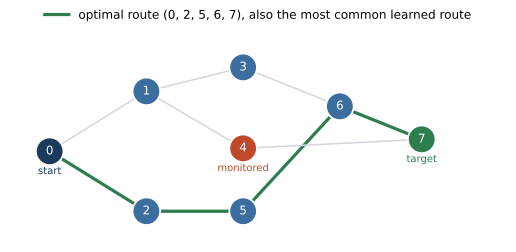
Figure 6.8. The eight-host network of the lab as an MDP. The agent starts at host 0 and seeks the target, host 7, while host 4 is monitored and carries a detection penalty. Edges join neighboring hosts, between which moves are possible. The green path is the optimal route found by value iteration, which avoids the monitored host; it is also the route learned by the largest number of Q-learning seeds. Produced by Lab 6c.
Return, discount and value functions
The agent does not maximize the immediate reward but the return, the discounted sum of future rewards from a time \(t\),
where the discount factor \(\gamma \in [0, 1)\) weights nearer rewards more heavily and keeps the sum finite when rewards are bounded. A discount near one makes the agent far-sighted; a smaller discount makes it prefer reward sooner, which in the lab, with \(\gamma = 0.95\), favors shorter paths to the target.
Two value functions summarize how good a situation is under a policy \(\pi\). The state-value \(V^\pi(s)\) is the expected return from state \(s\), and the action-value \(Q^\pi(s, a)\) is the expected return from taking action \(a\) in state \(s\) and following \(\pi\) thereafter,
The optimal action-value \(Q^\star(s, a)\) is the largest action-value achievable by any policy. It satisfies the Bellman optimality equation, which relates the value of a state-action pair to the values of its successors,
The optimal policy acts greedily with respect to \(Q^\star\), choosing \(\arg\max_a Q^\star(s, a)\) in each state. When the transition rule and rewards are known, as in the lab, equation \eqref{eq:bellman} can be solved directly by value iteration, which gives a reference policy to check learning against.
Show the answer
On the safe route the only reward is \(+1\) on the fourth move, so \(G_0 = \gamma^3 = 0.95^3 = 0.857\). On the other route the second move enters the monitored host. With probability 0.9 the episode ends there with reward \(-1\), contributing \(\gamma \times (-1) = -0.95\), and with probability 0.1 the agent continues and reaches the target on the third move, contributing \(\gamma^2 = 0.9025\). The expected return is \(0.9 \times (-0.95)\) plus \(0.1 \times 0.9025\), which equals \(-0.765\). The extra move of the safe route costs only a factor of 0.95, while the detection penalty dominates the shorter route, so the optimal policy avoids the monitored host.
Q-learning
Reinforcement learning is needed when the transition rule and rewards are not known in advance and must be learned from experience. Q-learning (Watkins and Dayan, 1992) estimates \(Q^\star\) from observed transitions without a model. After taking action \(a_t\) in state \(s_t\) and observing reward \(r_{t+1}\) and next state \(s_{t+1}\), it updates
where the learning rate \(\alpha \in (0, 1]\) controls how much each new experience moves the estimate. The bracketed quantity is the temporal-difference error, the gap between the current estimate and a one-step-ahead target built from the observed reward and the best next-state value. Watkins and Dayan (1992) proved that, for a finite MDP with bounded rewards, these estimates converge to \(Q^\star\) with probability one, provided every state-action pair is tried infinitely often and the learning rates decrease appropriately (their sum diverges while the sum of their squares stays finite).
A worked example shows the update propagating value backward. Take \(\alpha = 0.5\) and \(\gamma = 0.95\), with all action-values starting at zero. The first time the agent takes an action from a state \(s\) that reaches the target, with reward \(1\) and no successor because the episode ends, equation \eqref{eq:qlearning} gives \(Q \leftarrow 0 + 0.5(1 - 0) = 0.5\). Later, an action that leads from a predecessor state to \(s\) with reward \(0\) is updated. Since now \(\max_a Q(s, a) = 0.5\), its target is \(0 + 0.95 \times 0.5 = 0.475\), and the update is \(Q \leftarrow 0 + 0.5(0.475 - 0)\), which equals \(0.2375\). The reward at the target has begun to flow back to the states that lead to it, one step per update.
Exploration and the tie-breaking pitfall
To discover which actions are good, the agent must sometimes try actions that currently look suboptimal. The common rule is epsilon-greedy. With probability \(1 - \varepsilon\) choose the greedy action \(\arg\max_a Q(s, a)\), and with probability \(\varepsilon\) choose a uniformly random action. A larger \(\varepsilon\) explores more but earns less while doing so.
There is a subtle trap in how the greedy action is chosen. Before the agent has learned anything, all action-values are equal, so \(\arg\max_a Q(s, a)\) is a tie. A standard \(\arg\max\) that always returns the first maximal index resolves every such tie toward the same action. An untrained agent then repeats that one action in every state, and only the small \(\varepsilon\) fraction of steps tries anything else. When the reward is sparse and lies at the end of a particular path, this bias can keep the agent from reaching the reward often enough to learn anything. The remedy is to break ties at random, or to initialize the action-values optimistically so that every untried action looks attractive and gets tried, as Sutton and Barto (2018) discuss. This is a mechanical detail with a decisive effect, and it is worth stating because an agent that fails to learn here is easy to misdiagnose as a problem with the reward or the environment.
The lab demonstrates both exploration effects. Figure 6.9 compares random tie-breaking with the first-index rule on the same MDP, with action-values starting at zero. The random-tie-breaking agent reaches a mean return of about 0.72 over its final 200 episodes, while the first-index agent stays near zero (-0.002). The first-index agent reaches the target in only 5 of its 15,000 training episodes across all seeds, too rarely for the reward to propagate back to the start host, so its estimated value of the start state remains 0.00 and it learns no route to the target. This is the failure mode described above, reproduced deliberately so you can see it.
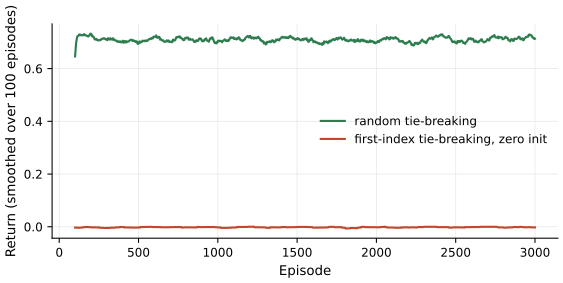
Figure 6.9. Discounted return per episode, averaged over five seeds and smoothed with a moving average over 100 episodes, on the lab MDP. The green curve uses random tie-breaking and rises as the agent learns the route; it stays below the exact optimal start value because the exploration rate of 0.1 keeps taking random actions. The red curve uses a deterministic first-index argmax with action-values initialized to zero and stays near zero, because the greedy choice out of a tie is always the same action. Produced by Lab 6c.
The exploration rate itself trades learning against earning. Figure 6.10 shows the mean final return as \(\varepsilon\) varies. On this MDP random tie-breaking alone supplies enough exploration, so even \(\varepsilon = 0\) learns the route, and the realized return falls as \(\varepsilon\) grows, from about 0.77 at \(\varepsilon = 0\) to about 0.29 at \(\varepsilon = 0.6\), because a large exploration rate spends many steps on random actions. With the deterministic first-index rule, by contrast, a positive \(\varepsilon\) is the only source of exploration. With \(\varepsilon = 0\) that agent would choose action 0 at the start host forever, a wasted step that never leaves the host.
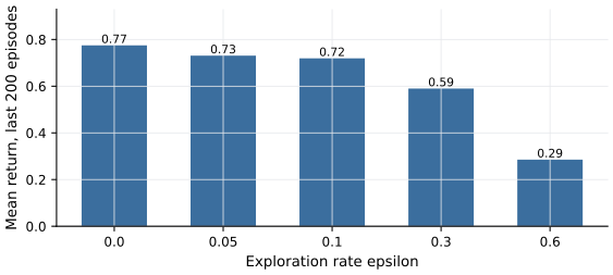
Figure 6.10. Mean discounted return over the last 200 of 3000 training episodes as a function of the exploration rate epsilon, with random tie-breaking, averaged over 3 seeds. Larger epsilon spends more steps on random actions and lowers the realized return on this MDP. Produced by Lab 6c.
The trained agent recovers a safe route. The exact optimal value of the start state, computed by value iteration, is 0.773. The learned greedy route equals the optimal route through hosts 2, 5 and 6 for 3 of 5 seeds, and the other seeds take the other safe route, through hosts 1, 3 and 6. The exact action-value of that route's first move, \(Q^\star(0, 1)\), is 0.766. This is the value of moving to host 1 and acting optimally afterwards, slightly below the optimum. The agent's own estimate of the start value, the largest of its action-values at the start host averaged over seeds, is 0.818, and it exceeds the exact optimum in 5 of 5 seeds. This is an instance of maximization bias (Sutton and Barto, 2018). The learning rate stays at 0.5, so each action-value keeps moving with the most recent sampled transitions instead of settling at its expectation, and a maximum taken over several such noisy estimates, as in the target of \eqref{eq:qlearning} and in reading out the start value, is biased upward. A decreasing learning rate shrinks the noise, and double Q-learning, which uses one set of estimates to choose the maximizing action and another to evaluate it, reduces the bias (Sutton and Barto, 2018).
Show the answer
The transition is terminal, so there is no successor term, and \eqref{eq:qlearning} gives \(Q \leftarrow 0 + 0.5(-1 - 0) = -0.5\). The action that enters the monitored host now has a negative value, so the greedy policy prefers any other action with value above \(-0.5\), steering the agent away from the monitored host.
Deep Q-networks
Tabular Q-learning stores one value per state-action pair, which is impossible when states are too many to enumerate. A deep Q-network (DQN) replaces the table with a neural network that maps a state to action-values. Training such a network naively can be unstable, because consecutive observations are correlated and the target in \eqref{eq:qlearning} shifts as the network changes. Mnih et al. (2015) stabilized it with two ideas: experience replay, which stores past transitions and samples them in random minibatches to break correlations, and a separate target network whose weights are held fixed for a number of updates and used to compute the targets, so the target does not chase the network at every step. With these, a single architecture with one set of hyperparameters learned to play 49 Atari 2600 games from screen pixels and the game score, reaching more than 75% of a professional human tester's score on 29 of them.
Security uses, reward hacking, and alignment
Reinforcement learning appears in security mainly through simulators. CybORG (Standen et al., 2021) is a gym for autonomous cyber operations that provides both a simulation and an emulation environment with a common interface, so an agent trained in simulation can be tested against a more realistic system. The network attack simulator of Schwartz and Kurniawati (2019) frames penetration testing as an MDP with the network configuration as state and scans and exploits as actions; in the simulator, tabular and neural-network Q-learning found optimal attack paths for a range of topologies, but the authors report that their implementations were practical only for smaller networks and would not scale to truly large ones. The realistic scope is that these are results in simulators on bounded problems, useful for studying planning agents, not evidence that an agent can autonomously penetrate an arbitrary real network.
Reinforcement learning also has a characteristic failure that matters for security. An agent optimizes the reward it is given, not the outcome the designer intended, so a poorly specified reward can be maximized in unintended ways. Amodei et al. (2016) call this reward hacking and list it among concrete problems in building systems that behave as intended. A defender who rewards an agent for closing alerts, for example, might find it closing them without resolving the underlying issue.
Finally, reinforcement learning is one of the methods used to align language models with human preferences. In reinforcement learning from human feedback, a reward model is trained from human comparisons of outputs and then used as the reward signal to fine-tune the model (Christiano et al., 2017; Ouyang et al., 2022). This is one widely used method among several, not the only way language models are aligned, and Unit 10 returns to it in the context of language-model security.
What the lab shows
Lab 6c
Open in ColabRead with outputsNotebook on GitHubAbout 1 minute to run on a laptop CPU
In Lab 6c you build the eight-host MDP, solve it exactly for reference, and train tabular Q-learning with random tie-breaking, recovering a safe route, the optimal route of Figure 6.8 for most seeds. You then vary \(\varepsilon\) and reproduce the tie-breaking failure of Figure 6.9, watching the first-index agent learn nothing while the random-tie-breaking agent succeeds.
Summary
Reinforcement learning fits a policy for acting in an MDP to maximize the discounted return of equation \eqref{eq:return}, using value functions and the Bellman optimality equation \eqref{eq:bellman}. Q-learning estimates the optimal action-values from experience with the update in equation \eqref{eq:qlearning}, exploring with an epsilon-greedy rule. The way ties in the greedy choice are broken can decide whether learning succeeds. A first-index argmax with zero-initialized values can keep an agent from reaching a sparse reward often enough to learn. The lab shows directly that random tie-breaking fixes it, and optimistic initialization is another remedy. Deep Q-networks scale the method with a function approximator, experience replay and a target network. In security, reinforcement learning is studied in simulation and emulation environments such as CybORG and in simulators such as the network attack simulator of Schwartz and Kurniawati, with bounded, carefully reported scope. It is vulnerable to reward hacking, and it underlies one common method for aligning language models.
References
- Amodei, D., Olah, C., Steinhardt, J., Christiano, P., Schulman, J., and Mané, D. (2016). Concrete problems in AI safety. arXiv. arXiv preprint arXiv:1606.06565. https://arxiv.org/abs/1606.06565
- Christiano, P. F., Leike, J., Brown, T. B., Martic, M., Legg, S., and Amodei, D. (2017). Deep reinforcement learning from human preferences. Advances in Neural Information Processing Systems, 30. https://proceedings.neurips.cc/paper_files/paper/2017/hash/d5e2c0adad503c91f91df240d0cd4e49-Abstract.html
- Mnih, V., Kavukcuoglu, K., Silver, D., Rusu, A. A., Veness, J., Bellemare, M. G., Graves, A., Riedmiller, M., Fidjeland, A. K., Ostrovski, G., Petersen, S., Beattie, C., Sadik, A., Antonoglou, I., King, H., Kumaran, D., Wierstra, D., Legg, S., and Hassabis, D. (2015). Human-level control through deep reinforcement learning. Nature, 518(7540), 529-533. https://doi.org/10.1038/nature14236
- Ouyang, L., Wu, J., Jiang, X., Almeida, D., Wainwright, C., Mishkin, P., Zhang, C., Agarwal, S., Slama, K., Ray, A., Schulman, J., Hilton, J., Kelton, F., Miller, L., Simens, M., Askell, A., Welinder, P., Christiano, P. F., Leike, J., and Lowe, R. (2022). Training language models to follow instructions with human feedback. Advances in Neural Information Processing Systems, 35, 27730-27744. https://proceedings.neurips.cc/paper_files/paper/2022/hash/b1efde53be364a73914f58805a001731-Abstract-Conference.html
- Schwartz, J., and Kurniawati, H. (2019). Autonomous penetration testing using reinforcement learning. University of Queensland. Bachelor of Science (Honours) thesis; arXiv preprint arXiv:1905.05965. https://arxiv.org/abs/1905.05965
- Standen, M., Lucas, M., Bowman, D., Richer, T. J., Kim, J., and Marriott, D. (2021). CybORG: A gym for the development of autonomous cyber agents. IJCAI-21 1st International Workshop on Adaptive Cyber Defense. arXiv preprint arXiv:2108.09118. https://arxiv.org/abs/2108.09118
- Sutton, R. S., and Barto, A. G. (2018). Reinforcement Learning: An Introduction. MIT Press, second edition. http://incompleteideas.net/book/the-book-2nd.html
- Watkins, C. J. C. H., and Dayan, P. (1992). Q-learning. Machine Learning, 8(3-4), 279-292. https://doi.org/10.1007/BF00992698