Unit 6 · Lesson 6.2
Sequence models for logs
System logs are a sequence. Each line records an event, and the order of events carries meaning. A privileged action that follows a granted privilege request is ordinary; the same privileged action with no preceding authorization is not. A detector that treats log lines as an unordered bag of features throws away that order. This lesson builds models that read a log as a sequence of event templates and predict what should come next, flagging anything surprising. It develops the n-gram baseline, recurrent networks and the vanishing-gradient problem that limits them, the long short-term memory (LSTM) cell that mitigates it, and the DeepLog approach to anomaly detection. It also states carefully what a sequence model adds over an ordinary classifier, because ordinary classifiers can use order too.
Logs as sequences of event templates
Raw log lines contain variable parts such as timestamps, identifiers and addresses. Log parsing replaces each line with a template, the constant part of the message, and treats the variable parts as parameters. For example the lines "Received block blk_3587 of size 67108864" and "Received block blk_9921 of size 33554432" share the template "Received block * of size *". A parser such as Drain (He et al., 2017) assigns each distinct template an integer key, so a log file becomes a sequence of keys drawn from a finite vocabulary. The models in this lesson operate on that sequence of keys.
A next-event model estimates the probability of the next key given a short history of recent keys. Writing \(k_t\) for the key at position \(t\) and a window of the \(w\) most recent keys as the history, the model estimates, for each key \(v\) in the vocabulary,
To detect anomalies, the keys are sorted by their predicted probability and the actual next key is treated as normal if it falls among the \(g\) most probable, called the top-g candidates, and flagged otherwise. A whole sequence is flagged if any of its events is flagged. Du et al. (2017) introduced this rule in DeepLog. Figure 6.5 illustrates the window and the top-g decision.
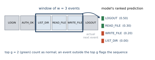
Figure 6.5. A sliding window of the last w = 3 events (blue) feeds a next-event model, which outputs a probability for each possible next event. The events are ranked; the top g = 2 (green) count as normal and the rest (red) would flag the sequence. The probabilities shown are those of the Lab 6b workflow after WRITE_FILE, so the actual next event, LOGOUT, ranks first and this position is normal. An event outside the top g at any position flags the whole sequence. Drawn as a schematic, following the DeepLog decision rule.
The parameter \(g\) sets the tradeoff. A small \(g\) is strict and flags more sequences, raising recall and lowering precision; a large \(g\) is permissive. The threshold plays the same role as the alert threshold of Unit 2, and it is chosen against an alert budget.
The n-gram baseline
The simplest next-event model counts. An n-gram model estimates \eqref{eq:nextevent} by the empirical frequency of each continuation of the history in the training data,
Here the history length \(w\) is the order of the model. This baseline is fast and can be strong. On their benchmark, Du et al. (2017) report that an n-gram model performs well with a history of one event but that its performance drops sharply as the history grows. Its weakness is that it has no estimate for a history it never saw during training, since the denominator of \eqref{eq:ngram} is zero, and the continuation is treated as unseen. For a vocabulary of any size the number of possible histories grows as the vocabulary raised to the power \(w\), so long histories are rarely all observed, and the model becomes brittle exactly when more context would help.
Recurrent networks and the vanishing-gradient problem
A recurrent neural network (RNN) reads a sequence one element at a time and maintains a hidden state that summarizes what it has seen. At step \(t\) it updates the state from the previous state and the current input, \(h_t = \phi(W h_{t-1} + U x_t + b)\), and predicts the next event from \(h_t\). Here \(x_t\) is the input vector at step \(t\) (for a log, a vector representing the key \(k_t\)), \(W\) and \(U\) are learned weight matrices, \(b\) is a learned bias vector and \(\phi\) is an elementwise activation such as \(\tanh\). In principle the state can carry information from arbitrarily far back, so an RNN is not limited to a fixed window like the n-gram model.
In practice training an RNN to use distant context is hard. The gradient of a loss at step \(t\) with respect to a state many steps earlier is a product of many factors, one per step, and such a product tends either to zero or to infinity as the number of steps grows. Bengio et al. (1994) showed why gradient descent struggles to learn long-term dependencies. In their analysis a recurrent system that stores information reliably for a long time has gradients that vanish over that time, a tradeoff between latching information for long periods and learning efficiently by gradient descent. A simple numeric view makes the effect concrete. If each step multiplies the backpropagated gradient by a factor of about 0.7, then after 20 steps the gradient is scaled by \(0.7^{20} \approx 0.000798\), which vanishes; if the factor is 1.3, the scale is \(1.3^{20} \approx 190\), which explodes. Either way the gradient at a distant step carries little usable signal.
Show the answer
The scale is \(0.8^{30} \approx 0.00124\). The gradient reaching the decisive early event is about one thousandth of its original size, so the network receives almost no training signal for that long-range dependency. This is the vanishing-gradient problem that motivates gated architectures.
LSTM gates
The long short-term memory cell of Hochreiter and Schmidhuber (1997) addresses vanishing gradients by adding a cell state that is updated mostly by addition rather than repeated multiplication, together with multiplicative gates that control what enters the cell state and what is read from it. The original design had an input gate and an output gate; the forget gate, which lets the cell discard stored information, was added by Gers et al. (2000). Writing \([h_{t-1}, x_t]\) for the concatenation of the previous output and the current input, the cell computes
where \(\sigma\) is the logistic sigmoid, \(W_f\), \(W_i\), \(W_o\) and \(b_f\), \(b_i\), \(b_o\) are the learned weight matrices and bias vectors of the gates, and \(f_t\), \(i_t\), \(o_t\) are the forget, input and output gates, each with entries in \((0, 1)\). A candidate update and the new cell and output states are
where \(W_c\) and \(b_c\) are the weight matrix and bias vector of the candidate and \(\odot\) is elementwise multiplication. These equations are the form implemented in current deep-learning libraries, including the PyTorch LSTM used in Lab 6b. The original papers squash the cell input and output with scaled logistic functions in place of the two \(\tanh\) functions, and they let several cells in a memory block share one set of gates, which does not change the mechanism. The forget gate scales the old cell state, the input gate scales the candidate, and the output gate scales what is read out. When the forget gate is near one and the input gate near zero, the cell state passes through almost unchanged, which lets information and gradients flow across many steps. Figure 6.6 shows the arrangement.
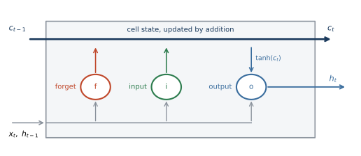
Figure 6.6. An LSTM cell. The cell state c runs along the top with mostly additive updates, the path that preserves information across many steps. The forget gate f, input gate i and output gate o, computed from the current input and previous output by equation \eqref{eq:lstm-gates}, control what the cell discards, stores and reads out. Drawn as a schematic.
A single scalar cell makes the arithmetic checkable. Take an input \(x_t = 1\), previous output \(h_{t-1} = 0\) and previous cell state \(c_{t-1} = 0.5\), with weights chosen so that the gate pre-activations are \(1.4\) for the forget gate, \(0.4\) for the input gate, \(0.9\) for the output gate and \(1.0\) for the candidate. Then \(f_t = \sigma(1.4) = 0.8022\), \(i_t = \sigma(0.4) = 0.5987\), \(o_t = \sigma(0.9) = 0.7109\) and \(\tilde{c}_t = \tanh(1.0) = 0.7616\). By equation \eqref{eq:lstm-state}, the new cell state and output are
The high forget gate keeps most of the old cell state while the input gate admits part of the new candidate.
Show the answer
The forget gate becomes \(f_t = \sigma(-2) = 0.1192\), so
The cell has discarded almost all of its old state, which now contributes 0.0596 instead of 0.4011, and the new cell state consists mostly of the admitted candidate. This is the reset behavior that the forget gate of Gers et al. (2000) was introduced to provide.
The gated recurrent unit (GRU) of Cho et al. (2014) is a simpler variant with two gates, an update gate that interpolates between the old state and a candidate and a reset gate that controls how much past state enters the candidate, with no separate cell state. With three sets of weights instead of the LSTM's four, it has fewer parameters than an LSTM of the same width.
DeepLog and what sequence models add
DeepLog (Du et al., 2017) trains an LSTM next-event model on normal log sequences only and applies the top-g rule to its estimate of \eqref{eq:nextevent}. Because it learns from normal behavior alone, it needs no labeled attacks, which suits a setting where normal operation is abundant and attacks are rare and varied. Unlike the n-gram model, the LSTM shares information across histories through its hidden state, so a history it never saw exactly can still receive a sensible prediction.
It is tempting to say that only a sequence model can use order, but that is not accurate. An ordinary classifier can be given order through features: counts within a sliding window, the identity of the previous one or two events (lag features), or n-gram indicators. What a recurrent model adds is the ability to summarize a variable-length history in a learned state and to generalize across histories, rather than relying on a fixed set of hand-chosen window or lag features. The useful comparison is therefore between a model that learns its own summary of the past and one given a fixed, human-designed summary.
Transformers, which Unit 10 covers, are the main alternative to recurrent models for sequences. They replace recurrence with an attention mechanism that lets every position attend to every other, which shortens the path between distant positions and allows training in parallel (Vaswani et al., 2017). A note of caution applies to all of these models. Le and Zhang (2022) re-evaluated several deep log-anomaly detectors and found that the results depend strongly on how the training data are selected, how log events are grouped into sequences, the class balance and the noise in the data, and they conclude that log-based anomaly detection has not been solved. A high score on one benchmark does not transfer automatically to a new system's logs.
What the lab shows
Lab 6b
Detecting anomalous log sequences with an LSTM
Open in ColabRead with outputsNotebook on GitHubAbout 1 minute to run on a laptop CPU
In Lab 6b you generate synthetic log sequences from a stochastic workflow, inject three kinds of anomalies, and compare an n-gram model with a history of 3 events against an LSTM next-event model that reads the whole prefix of each sequence. The sequences are synthetic because labeled security-log datasets are scarce and system specific, and a generator lets you control exactly which anomalies are present. The lab keeps an out-of-order swap only when the swapped sequence contains a transition that the workflow cannot produce, so every sequence labeled anomalous really is one and precision and recall are meaningful. Figure 6.7 shows how recall and precision change as the top-g threshold grows. At \(g = 2\) the LSTM flags anomalies with recall 1.00, but it also flags most normal sequences, because many normal transitions have probability 0.2 or 0.3 and fall outside the top two, so its precision is only 0.29 (the n-gram model reaches recall 1.00 at precision 0.25). At \(g = 4\), the largest number of successors any event has in the workflow, neither model flags a normal sequence, so both reach precision 1.00. The n-gram model keeps recall 1.00 there, while the LSTM's recall falls to 0.95.
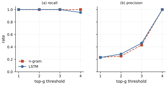
Figure 6.7. Recall (a) and precision (b) of the n-gram and LSTM next-event detectors as the top-g threshold varies from 1 to 4, on a test set of 2,000 held-out normal sequences and 600 injected anomalies. A larger g is more permissive, so recall can only stay level or fall; on this test set precision rises. Produced by Lab 6b.
The table below gives recall per anomaly kind at \(g = 4\), the operating point at which neither model flags a normal sequence. Both models catch every rare-transition and privileged-without-authorization anomaly. They differ on the out-of-order anomalies. The LSTM's top g always contains g events, so after an event with fewer than g possible successors (LOGIN has one, AUTH_OK three) it also accepts events that the workflow never produces at that point, and some swaps pass unflagged. The n-gram model ranks only continuations it has observed after the current history, so it rejects every continuation it never saw after that history in training.
| Anomaly kind | n-gram recall | LSTM recall |
|---|---|---|
| out-of-order step | 1.00 | 0.86 |
| rare transition | 1.00 | 1.00 |
| privileged step without authorization | 1.00 | 1.00 |
In this workflow the next event depends only on the current one, so a short n-gram history is the correct model. The counting baseline has recall at least as high as the LSTM at every g, and at \(g = 4\), where neither model flags a normal sequence, it matches the LSTM on two anomaly kinds and beats it on the third. At \(g = 2\) and \(g = 3\) both models catch every anomaly, and the LSTM flags fewer normal sequences, so its precision is slightly higher there. This agrees with the strength of the short-history n-gram baseline that Du et al. (2017) report. The ability of the LSTM to generalize across histories would matter for dependencies that reach further back than any history the n-gram model can afford to count.
Summary
A log becomes a sequence of event-template keys, and a next-event model estimates the distribution of the next key from a recent history, flagging any event outside the top g. An n-gram model estimates this by counting and can be strong at short histories, but it has nothing to say about histories it never saw. Recurrent networks can in principle carry distant context, but the vanishing-gradient problem makes long-range learning hard, which the LSTM mitigates with an additive cell state and multiplicative gates defined in equations \eqref{eq:lstm-gates} and \eqref{eq:lstm-state}. DeepLog applies an LSTM next-event model trained on normal logs with the top-g rule. Plain classifiers can use order through window, lag or n-gram features, and what a sequence model adds is a learned summary of a variable-length history. On the lab's first-order workflow the counting baseline has recall at least as high as the LSTM at every g and outperforms it at \(g = 4\), where neither model flags a normal sequence, while the LSTM has slightly higher precision at \(g = 2\) and \(g = 3\). Transformers are the main alternative to recurrent models, and careful evaluation remains necessary because benchmark accuracy does not transfer automatically to a new system.
References
- Bengio, Y., Simard, P., and Frasconi, P. (1994). Learning long-term dependencies with gradient descent is difficult. IEEE Transactions on Neural Networks, 5(2), 157-166. https://doi.org/10.1109/72.279181
- Cho, K., van Merrienboer, B., Gulcehre, C., Bahdanau, D., Bougares, F., Schwenk, H., and Bengio, Y. (2014). Learning phrase representations using RNN encoder-decoder for statistical machine translation. Proceedings of the 2014 Conference on Empirical Methods in Natural Language Processing (EMNLP), 1724-1734. https://doi.org/10.3115/v1/D14-1179
- Du, M., Li, F., Zheng, G., and Srikumar, V. (2017). DeepLog: Anomaly detection and diagnosis from system logs through deep learning. Proceedings of the 2017 ACM SIGSAC Conference on Computer and Communications Security (CCS), 1285-1298. https://doi.org/10.1145/3133956.3134015
- Gers, F. A., Schmidhuber, J., and Cummins, F. (2000). Learning to forget: Continual prediction with LSTM. Neural Computation, 12(10), 2451-2471. https://doi.org/10.1162/089976600300015015
- He, P., Zhu, J., Zheng, Z., and Lyu, M. R. (2017). Drain: An online log parsing approach with fixed depth tree. 2017 IEEE International Conference on Web Services (ICWS), 33-40. https://doi.org/10.1109/ICWS.2017.13
- Hochreiter, S., and Schmidhuber, J. (1997). Long short-term memory. Neural Computation, 9(8), 1735-1780. https://doi.org/10.1162/neco.1997.9.8.1735
- Le, V.-H., and Zhang, H. (2022). Log-based anomaly detection with deep learning: How far are we?. Proceedings of the 44th International Conference on Software Engineering (ICSE), 1356-1367. https://doi.org/10.1145/3510003.3510155
- Vaswani, A., Shazeer, N., Parmar, N., Uszkoreit, J., Jones, L., Gomez, A. N., Kaiser, Ł., and Polosukhin, I. (2017). Attention is all you need. Advances in Neural Information Processing Systems, 30. https://proceedings.neurips.cc/paper_files/paper/2017/hash/3f5ee243547dee91fbd053c1c4a845aa-Abstract.html