Unit 6 · Lab 6a
A convolutional network and transfer learning
Lab 6a
A convolutional network and transfer learning
Open in ColabRead with outputsNotebook on GitHubAbout 3 minutes to run on a laptop CPU
# On Google Colab, install the scikit-learn version the course was built with.
# On your own computer, install requirements.txt instead; this cell then does nothing.
import subprocess, sys
if "google.colab" in sys.modules:
    subprocess.run([sys.executable, "-m", "pip", "install", "-q", "scikit-learn==1.9.0"], check=True)
Lab 6a. A convolutional network and transfer learning
This lab has two parts. First it trains a small convolutional network (CNN) on a subset of MNIST, counts its parameters layer by layer, and plots its eight first-layer filters and the feature maps they produce. Second it studies transfer learning on CIFAR-10, comparing a frozen ResNet-18 feature extractor followed by logistic regression with a small network trained from scratch as the number of labeled training images grows. Everything runs on CPU within a few minutes.
You will:
- train a small CNN on an MNIST subset and read off its parameter count by layer;
- visualize the first-layer filters and the feature maps they produce;
- extract pretrained ResNet-18 features from CIFAR-10 images and classify them with logistic regression;
- train a small CNN from scratch on the same CIFAR-10 subsets;
- plot accuracy against the number of labeled images for both approaches, averaged over seeds.
MNIST and CIFAR-10 are standard image datasets. They stand in for the image-shaped security data of Lesson 6.1, such as malware byte-plots, because they are small, labeled and well understood. The learning mechanics are identical.
import os
import warnings

import numpy as np
import matplotlib.pyplot as plt
import torch
import torch.nn as nn
import torch.nn.functional as F
from sklearn.linear_model import LogisticRegression
from torchvision import transforms
from torchvision.datasets import MNIST, CIFAR10
import torchvision.models as models

warnings.filterwarnings("ignore", category=UserWarning)
torch.set_num_threads(4)
SEED = 20251015
torch.manual_seed(SEED)
rng = np.random.default_rng(SEED)
ROOT = "../../data/downloads"
1. A small CNN on MNIST
We take a balanced subset of MNIST to keep training fast. The network has two convolutional layers, each followed by max pooling, then two fully connected layers. Max pooling keeps the largest activation in each 2 by 2 window, which lowers the resolution and makes the features less sensitive to small shifts.
mnist_train = MNIST(root=ROOT, train=True, download=True)
mnist_test = MNIST(root=ROOT, train=False, download=True)
Xtr = (mnist_train.data.numpy().astype(np.float32) / 255.0)
ytr = mnist_train.targets.numpy()
Xte = (mnist_test.data.numpy().astype(np.float32) / 255.0)
yte = mnist_test.targets.numpy()

# Balanced subset: 600 training and 200 test images per digit.
def balanced_subset(X, y, per_class, seed):
    r = np.random.default_rng(seed)
    idx = []
    for c in range(10):
        pool = np.flatnonzero(y == c)
        idx.extend(r.choice(pool, per_class, replace=False))
    idx = np.array(idx)
    r.shuffle(idx)
    return X[idx], y[idx]

Xm, ym = balanced_subset(Xtr, ytr, 600, SEED)
Xmte, ymte = balanced_subset(Xte, yte, 200, SEED + 1)
Xm_t = torch.from_numpy(Xm).unsqueeze(1)
ym_t = torch.from_numpy(ym).long()
Xmte_t = torch.from_numpy(Xmte).unsqueeze(1)
print(f"MNIST subset: {len(Xm)} train, {len(Xmte)} test")


class SmallCNN(nn.Module):
    def __init__(self, in_ch=1, n_classes=10, hw=28):
        super().__init__()
        self.conv1 = nn.Conv2d(in_ch, 8, kernel_size=3, padding=1)
        self.conv2 = nn.Conv2d(8, 16, kernel_size=3, padding=1)
        flat = 16 * (hw // 4) * (hw // 4)
        self.fc1 = nn.Linear(flat, 64)
        self.fc2 = nn.Linear(64, n_classes)

    def features(self, x):
        a1 = F.relu(self.conv1(x))
        p1 = F.max_pool2d(a1, 2)
        a2 = F.relu(self.conv2(p1))
        p2 = F.max_pool2d(a2, 2)
        return a1, p1, a2, p2

    def forward(self, x):
        _, _, _, p2 = self.features(x)
        z = p2.flatten(1)
        z = F.relu(self.fc1(z))
        return self.fc2(z)


cnn = SmallCNN()
MNIST subset: 6000 train, 2000 test
Parameter count by layer
The convolutional layers have few parameters because their weights are shared across all positions. The fully connected layers, which connect every input to every output, hold most of the parameters. The cell below lists each layer's count.
layer_params = {}
for name, p in cnn.named_parameters():
    layer_params[name] = int(p.numel())
by_layer = {}
for name, n in layer_params.items():
    key = name.split(".")[0]
    by_layer[key] = by_layer.get(key, 0) + n
total_params = sum(by_layer.values())
for k, n in by_layer.items():
    print(f"{k:<6} {n:>8,}  ({100 * n / total_params:.1f}%)")
print(f"{'total':<6} {total_params:>8,}")

conv_params = by_layer["conv1"] + by_layer["conv2"]
fc_params = by_layer["fc1"] + by_layer["fc2"]
# For comparison, a dense first layer mapping the 784 input pixels to the same number of
# first-layer feature values (8 channels at 28x28) would have this many parameters
# (weights and biases).
dense_equiv = (28 * 28) * (8 * 28 * 28) + (8 * 28 * 28)
print(f"conv layers: {conv_params:,}; fully connected: {fc_params:,}")
print(f"a dense layer producing the same first feature map: {dense_equiv:,} parameters")
conv1 80 (0.2%) conv2 1,168 (2.2%) fc1 50,240 (96.4%) fc2 650 (1.2%) total 52,138 conv layers: 1,248; fully connected: 50,890 a dense layer producing the same first feature map: 4,923,520 parameters
Train the CNN
A few epochs of Adam are enough on this subset to reach high accuracy.
def train_cnn(model, X, y, epochs=8, lr=3e-3, batch=128, seed=0):
    r = np.random.default_rng(seed)
    opt = torch.optim.Adam(model.parameters(), lr=lr)
    loss_fn = nn.CrossEntropyLoss()
    n = len(X)
    for ep in range(epochs):
        order = r.permutation(n)
        model.train()
        for i in range(0, n, batch):
            idx = order[i:i + batch]
            opt.zero_grad()
            loss = loss_fn(model(X[idx]), y[idx])
            loss.backward()
            opt.step()
    return model


@torch.no_grad()
def accuracy(model, X, y):
    model.eval()
    preds = model(X).argmax(1).numpy()
    return float((preds == y).mean())


train_cnn(cnn, Xm_t, ym_t, epochs=8, seed=SEED)
mnist_acc = accuracy(cnn, Xmte_t, ymte)
print(f"MNIST subset test accuracy: {mnist_acc:.3f}")
MNIST subset test accuracy: 0.967
2. Filters and feature maps
The first convolutional layer learns eight 3 by 3 filters. Each one slides over the image and responds to a small local pattern. The cell below extracts the eight filters and the feature map each of them produces on one example digit, a 7 from the test subset, and plots them. The digit is at the left, the filters are in the top row, and their feature maps are in the bottom row, where brighter means a stronger response.
filters = cnn.conv1.weight.detach().numpy()[:, 0, :, :]  # 8 filters, 3x3
example = Xmte_t[ymte == 7][0:1]  # a digit 7
a1, p1, a2, p2 = cnn.features(example)
fmaps = a1.detach().numpy()[0]  # 8 feature maps, 28x28
example_img = example.numpy()[0, 0]

fig, axes = plt.subplots(2, 9, figsize=(10, 2.6))
axes[0, 0].imshow(example_img, cmap="gray")
axes[1, 0].axis("off")
for k in range(8):
    axes[0, k + 1].imshow(filters[k], cmap="gray")
    axes[1, k + 1].imshow(fmaps[k], cmap="gray")
for ax in axes.flat:
    ax.set_xticks([])
    ax.set_yticks([])
plt.tight_layout()
plt.show()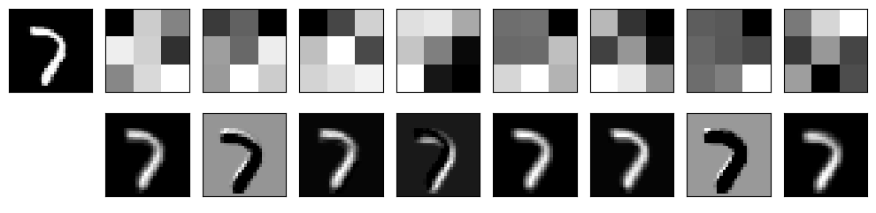
3. Transfer learning on CIFAR-10 with pretrained features
CIFAR-10, a set of small color photographs of ten object classes, is harder than MNIST. A network trained from scratch on a few hundred images overfits. Transfer learning reuses a network trained on a large dataset, here ImageNet; in this lab the pretrained network serves as a fixed feature extractor. We pass CIFAR-10 images through a pretrained ResNet-18 with its classification head removed, take the 512-dimensional output, and train a logistic regression on top. The ResNet weights never change, so this is the frozen feature extractor approach of Lesson 6.1.
cifar_train = CIFAR10(root=ROOT, train=True, download=True)
cifar_test = CIFAR10(root=ROOT, train=False, download=True)
Ctr = cifar_train.data  # (50000, 32, 32, 3) uint8
ctr = np.array(cifar_train.targets)
Cte = cifar_test.data
cte = np.array(cifar_test.targets)

# A fixed, balanced test set and a labeled pool to draw training subsets from.
pool_X, pool_y = balanced_subset(Ctr, ctr, 100, SEED)       # 1000 images, 100 per class
test_X, test_y = balanced_subset(Cte, cte, 200, SEED + 2)   # 2000 images, 200 per class

IMAGENET_MEAN = [0.485, 0.456, 0.406]
IMAGENET_STD = [0.229, 0.224, 0.225]
resnet_tf = transforms.Compose([
    transforms.ToTensor(),
    transforms.Resize(64, antialias=True),
    transforms.Normalize(IMAGENET_MEAN, IMAGENET_STD),
])


def to_resnet_batch(imgs):
    return torch.stack([resnet_tf(img) for img in imgs])


backbone = models.resnet18(weights=models.ResNet18_Weights.DEFAULT)
backbone.fc = nn.Identity()
backbone.eval()


@torch.no_grad()
def resnet_features(imgs, batch=200):
    feats = []
    for i in range(0, len(imgs), batch):
        x = to_resnet_batch(imgs[i:i + batch])
        feats.append(backbone(x).numpy())
    return np.concatenate(feats)


pool_feat = resnet_features(pool_X)
test_feat = resnet_features(test_X)
print(f"ResNet-18 features: pool {pool_feat.shape}, test {test_feat.shape}")
ResNet-18 features: pool (1000, 512), test (2000, 512)
4. A small CNN trained from scratch on CIFAR-10
For comparison we train the same style of small CNN directly on the raw 32 by 32 images, with no pretraining.
def cifar_tensors(imgs):
    x = imgs.astype(np.float32) / 255.0
    x = (x - np.array(IMAGENET_MEAN)) / np.array(IMAGENET_STD)
    return torch.from_numpy(x.transpose(0, 3, 1, 2)).float()


test_X_t = cifar_tensors(test_X)
test_y_np = test_y
5. Accuracy as a function of the number of labeled images
For each training size we draw a balanced subset from the labeled pool of 1000 images, train both methods, and record test accuracy, averaged over three seeds. At 1000 images the subset is the whole pool, so the seeds then differ only in the order of the images and, for the from-scratch network, in its initialization. The frozen-feature approach is expected to win by a wide margin when labels are scarce.
SIZES = [100, 300, 1000]
SEEDS = [0, 1, 2]
transfer_acc = {n: [] for n in SIZES}
scratch_acc = {n: [] for n in SIZES}

for n in SIZES:
    per_class = n // 10
    for sd in SEEDS:
        r = np.random.default_rng(1000 + sd)
        sel = []
        for c in range(10):
            pc = np.flatnonzero(pool_y == c)
            sel.extend(r.choice(pc, per_class, replace=False))
        sel = np.array(sel)

        clf = LogisticRegression(max_iter=2000, C=1.0)
        clf.fit(pool_feat[sel], pool_y[sel])
        transfer_acc[n].append(float((clf.predict(test_feat) == test_y).mean()))

        torch.manual_seed(sd)
        net = SmallCNN(in_ch=3, n_classes=10, hw=32)
        Xsub = cifar_tensors(pool_X[sel])
        ysub = torch.from_numpy(pool_y[sel]).long()
        train_cnn(net, Xsub, ysub, epochs=25, lr=3e-3, seed=sd)
        scratch_acc[n].append(accuracy(net, test_X_t, test_y_np))
    print(f"n={n:>4}  transfer {np.mean(transfer_acc[n]):.3f}  scratch {np.mean(scratch_acc[n]):.3f}")

fig, ax = plt.subplots(figsize=(6, 3.2))
for acc, label in [(transfer_acc, "frozen ResNet-18 features"),
                   (scratch_acc, "small CNN from scratch")]:
    ax.errorbar(SIZES, [np.mean(acc[n]) for n in SIZES],
                yerr=[np.std(acc[n]) for n in SIZES],
                marker="o", capsize=3, label=label)
ax.axhline(0.1, ls=":", color="gray", label="uniform guessing")
ax.set_xscale("log")
ax.set_xticks(SIZES, [str(n) for n in SIZES])
ax.minorticks_off()
ax.set_ylim(0, 0.8)
ax.set_xlabel("labeled training images")
ax.set_ylabel("test accuracy")
ax.legend()
plt.tight_layout()
plt.show()
n= 100 transfer 0.562 scratch 0.244
n= 300 transfer 0.614 scratch 0.326
n=1000 transfer 0.675 scratch 0.404
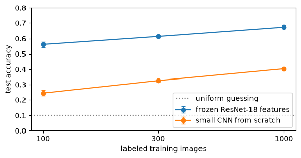
The cell above prints the mean accuracy of each method at each training size and plots both curves, with error bars showing the standard deviation across seeds. The frozen ResNet-18 features, classified by a simple logistic regression, reach higher accuracy than the from-scratch CNN at every size, and the gap is largest when labels are scarcest. This is the practical case for transfer learning in a security setting where labeled attack images are few.
Try this
- Replace the frozen features with the raw pixels (flatten the 32 by 32 by 3 image) and train logistic regression on those; compare the accuracy.
- Unfreeze the last ResNet block and fine-tune it on the 1000-image subset; does accuracy improve enough to justify the extra computation?
- Increase the from-scratch CNN to three convolutional layers and see whether it closes the gap at 1000 images.
Results summary
These are the numbers quoted in the lesson text.
results = {
    "mnist_train": int(len(Xm)),
    "mnist_test": int(len(Xmte)),
    "mnist_acc": float(mnist_acc),
    "total_params": int(total_params),
    "conv_params": int(conv_params),
    "fc_params": int(fc_params),
    "fc_fraction": float(fc_params / total_params),
    "conv1_params": int(by_layer["conv1"]),
    "conv2_params": int(by_layer["conv2"]),
    "fc1_params": int(by_layer["fc1"]),
    "fc2_params": int(by_layer["fc2"]),
    "dense_equiv_params": int(dense_equiv),
    "cifar_test": int(len(test_X)),
    "transfer_acc_100": float(np.mean(transfer_acc[100])),
    "transfer_acc_300": float(np.mean(transfer_acc[300])),
    "transfer_acc_1000": float(np.mean(transfer_acc[1000])),
    "scratch_acc_100": float(np.mean(scratch_acc[100])),
    "scratch_acc_300": float(np.mean(scratch_acc[300])),
    "scratch_acc_1000": float(np.mean(scratch_acc[1000])),
    "gap_100": float(np.mean(transfer_acc[100]) - np.mean(scratch_acc[100])),
}
for k, v in results.items():
    print(f"{k:<22} {v}")

export = {
    "sizes": SIZES,
    "transfer_mean": [float(np.mean(transfer_acc[n])) for n in SIZES],
    "transfer_std": [float(np.std(transfer_acc[n])) for n in SIZES],
    "scratch_mean": [float(np.mean(scratch_acc[n])) for n in SIZES],
    "scratch_std": [float(np.std(scratch_acc[n])) for n in SIZES],
    "filters": filters.tolist(),
    "feature_maps": fmaps.tolist(),
    "example_img": example_img.tolist(),
    "layer_names": ["conv1", "conv2", "fc1", "fc2"],
    "layer_counts": [int(by_layer[k]) for k in ["conv1", "conv2", "fc1", "fc2"]],
}

if os.environ.get("COURSE_RESULTS"):
    import json
    with open(os.environ["COURSE_RESULTS"], "w") as f:
        json.dump({"results": results, "data": export}, f)
mnist_train 6000 mnist_test 2000 mnist_acc 0.9665 total_params 52138 conv_params 1248 fc_params 50890 fc_fraction 0.9760635237254978 conv1_params 80 conv2_params 1168 fc1_params 50240 fc2_params 650 dense_equiv_params 4923520 cifar_test 2000 transfer_acc_100 0.5618333333333333 transfer_acc_300 0.6141666666666666 transfer_acc_1000 0.6746666666666666 scratch_acc_100 0.24433333333333332 scratch_acc_300 0.3261666666666667 scratch_acc_1000 0.4040000000000001 gap_100 0.3175