Unit 6 · Lesson 6.1
Convolutional networks and transfer learning
A fully connected network treats its input as a flat list of numbers and learns a separate weight for every input position. For an image, or for any security signal with a spatial or sequential layout, that is wasteful and fragile, because the same local pattern appearing in a new position looks entirely new to the model, and the number of weights grows with the input size. Convolutional networks replace the dense connection with a small filter that is applied at every position, which encodes the assumption that a useful local pattern is worth detecting wherever it occurs. This lesson develops the convolution operation and its arithmetic, counts the parameters it saves, explains what the architecture does and does not guarantee about shifts, and then turns to transfer learning, the practice of reusing a network trained on a large dataset as the starting point for a task with few labels. The security applications are malware images and detectors for synthetic media.
Convolution as a shared local filter
A convolutional layer stores a small set of weights called a filter or kernel and slides it across the input, computing a weighted sum at each location. Let the input be a stack of \(C_{\mathrm{in}}\) channels, written \(x[d, r, c]\) for channel \(d\) at row \(r\) and column \(c\). A layer with \(C_{\mathrm{out}}\) filters, each of size \(K \times K\), stride \(S\) and zero-padding \(P\), produces an output
where the sum runs over input channels \(d = 0, \ldots, C_{\mathrm{in}} - 1\) and filter offsets \(m, n = 0, \ldots, K - 1\), the weight \(w[k, d, m, n]\) belongs to filter \(k\) for input channel \(d\) at offset \((m, n)\), and \(b[k]\) is that filter's bias. Equation \eqref{eq:conv} is written for stride 1 with the padding folded into the input indexing; with a general stride \(S\) and padding \(P\) the input index becomes \(iS + m - P\) along each axis. The sum runs over the small \(K \times K\) window and over all input channels, so one output value depends only on a local region of the input, called its receptive field. The decisive property is that the same weights \(w[k, \cdot, \cdot, \cdot]\) appear in \eqref{eq:conv} for every output position \((i, j)\). This weight sharing is what distinguishes a convolution from a dense layer, in which each position would have its own weights. LeCun et al. (1998) describe convolutional networks as combining local receptive fields, shared weights and spatial subsampling, and present the network LeNet-5 built on these ideas. Figure 6.1 shows one filter evaluated at two positions and the pooling operation described below.
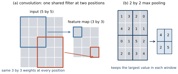
Figure 6.1. (a) A single 3 by 3 filter with one set of weights, evaluated at two positions of a 5 by 5 input (blue and red) to produce the corresponding entries of a 3 by 3 feature map. The same nine weights are used at every position. (b) Max pooling with 2 by 2 windows and stride 2, where each output is the largest of the four inputs in its window, here reducing a 4 by 4 map to 2 by 2. Drawn as a schematic.
The spatial size of the output follows from how many positions the window can occupy. Along one axis of length \(H_{\mathrm{in}}\),
With \(K = 3\), \(P = 1\) and \(S = 1\), equation \eqref{eq:outsize} gives \(H_{\mathrm{out}} = H_{\mathrm{in}}\), so the map keeps its size; this is the padding used in the lab. A stride larger than one skips positions and shrinks the output. After the weighted sum, a nonlinearity such as the rectified linear unit is applied elementwise.
Pooling reduces the spatial resolution between convolutional layers. Max pooling reports the largest activation in each pooling window (2 by 2 with stride 2 in the lab), as in Figure 6.1(b); average pooling reports the mean instead. Reducing resolution lowers the cost of later layers and makes the representation less sensitive to the exact position of a feature. Max pooling discards everything but the single strongest response in each window, while average pooling blends the whole window, so a description of pooling as keeping the strongest responses applies only to the maximum.
Show the answer
From equation \eqref{eq:outsize} with \(H_{\mathrm{in}} = 32\), \(K = 5\), \(P = 0\), \(S = 1\), the convolution gives \((32 - 5)/1 + 1 = 28\), so a 28 by 28 map. Max pooling with a 2 by 2 window and stride 2 halves each axis, giving 14 by 14.
Why convolution saves parameters, and where the parameters go
A convolutional layer has \(C_{\mathrm{out}}(C_{\mathrm{in}} K^2 + 1)\) weights, counting one bias per filter, and that count does not depend on the input's spatial size. The lab trains a small network on the MNIST handwritten-digit images (LeCun et al., 1998). Its first layer has eight 3 by 3 filters on a single input channel, so that layer has \(8 \times (1 \times 3 \times 3 + 1) = 80\) parameters. A dense layer that mapped the 784 input pixels to the same number of first-layer values, \(8 \times 28 \times 28 = 6272\) outputs, would need 4,923,520 weights (\(784 \times 6272 + 6272\)). The convolution achieves the same spatial coverage with almost five orders of magnitude fewer parameters, because it reuses one filter everywhere instead of learning a weight for every pair of positions.
Counting the parameters of the whole lab network is instructive, because the saving is not uniform. Figure 6.2 lists the four layers. The two convolutional layers together hold 1,248 parameters, while the fully connected layers hold 50,890, which is 97.6% of the 52,138 total. Almost all of that is in the first fully connected layer, which maps the flattened \(16 \times 7 \times 7 = 784\) values after the second pooling to 64 units, for 50,240 weights (\(784 \times 64 + 64\)). The lesson for a security practitioner sizing a model is that the convolutional feature extractor is cheap and the dense classifier on top is where the parameters, and the risk of overfitting a small labeled set, concentrate.
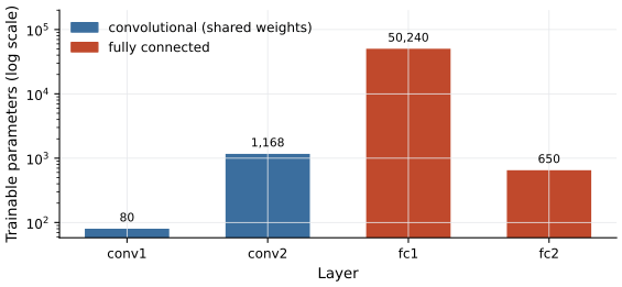
Figure 6.2. Trainable parameters per layer of the lab's MNIST network, on a logarithmic scale. The convolutional layers (blue) share weights and hold 1,248 parameters in total; the fully connected layers (red) hold 50,890, with 50,240 in the first of them alone. Produced by Lab 6a.
Equivariance, approximate invariance, and feature hierarchies
The convolution in \eqref{eq:conv} is translation equivariant. If the input is shifted by some amount, the output feature map is shifted by the same amount and is otherwise unchanged. Equivariance is a property of the operation and holds exactly for a stride-1 convolution, apart from effects at the border of the input; with stride \(S\) it holds only for shifts by multiples of \(S\). It is often loosely described as recognizing a pattern wherever it sits, but that phrasing conflates two different things. Equivariance means the response moves with the pattern; it does not by itself mean the network's final decision is unchanged when the input shifts.
Whether a whole convolutional network is invariant, giving the same output label under a shift, is a separate question. Pooling and strided layers build in some tolerance to small shifts, but Azulay and Weiss (2019) show that modern convolutional networks can change their prediction substantially under shifts or rescalings of a few pixels, because the subsampling steps ignore the sampling theorem and because data augmentation teaches invariance only for images close to the training distribution. For a security reader the practical consequence is that a detector operating on image-shaped data is only approximately invariant to such transformations, and an evaluation should test the transformations that matter rather than assume they are handled.
What the stacked layers learn is a hierarchy of features. First-layer filters of networks trained on natural images resemble oriented edge detectors (Gabor filters) and color blobs (Yosinski et al., 2014). Zeiler and Fergus (2014) visualized the features of deeper layers of a trained image network and found that the second layer responds to corners and other conjunctions of edges and colors, the third to similar textures, the fourth to more class-specific parts such as dog faces, and the fifth to entire objects. The lab makes a small version of this visible. Figure 6.3 shows the eight filters of the first layer and the feature maps they produce on one digit; the filters respond to oriented strokes, and most maps are darkest along those strokes, while two of them respond to the background and are near zero on the stroke itself.
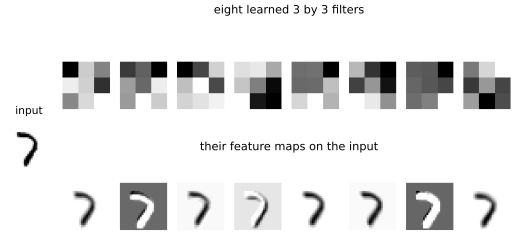
Figure 6.3. Left, an input digit from the MNIST test set. Top row, the eight learned 3 by 3 filters of the first convolutional layer, shown as grayscale weight patterns. Bottom row, the feature map each filter produces on the input, drawn, like the input, on a reversed gray scale, so darker means a stronger response. Different filters respond to differently oriented strokes. Produced by Lab 6a.
Transfer learning
Training a deep network from scratch needs many labeled examples, which a security team rarely has for a new threat. Transfer learning addresses this by reusing a network already trained on a large dataset. The lower layers of such a network compute general features that transfer to related tasks, while the upper layers are specific to the original task. Yosinski et al. (2014) quantified this transition from general to specific. They distinguish two ways of reusing the lower layers, either leaving them frozen, so their weights do not change on the new task, or fine-tuning them, so they continue to train, and note that the features are often left frozen when the target dataset is small and the transferred layers hold many parameters, because fine-tuning them then risks overfitting. Their experiments also found that initializing a network with transferred features improved generalization even after fine-tuning on the target dataset.
The lab shows the frozen case on CIFAR-10, a set of small color photographs in ten object classes (Krizhevsky, 2009). A ResNet-18 (He et al., 2016) pretrained on ImageNet is used, with its classification head removed, as a fixed feature extractor; a logistic regression is trained on the 512 features it outputs. This is compared with a small convolutional network trained from scratch on the same images, as the number of labeled training images grows. Figure 6.4 plots the result. With 2,000 test images and only 100 labeled training images, the frozen features reach 56.2% accuracy against 24.4% for the from-scratch network, so they classify correctly an additional 31.8% of the test images. The gap narrows as labels increase, to 67.5% against 40.4% at 1000 images, but the pretrained features remain ahead at every size tested. When labeled attack data is scarce, reusing features learned on a large related dataset can raise accuracy far above what the same few labels support when a network is trained from scratch.
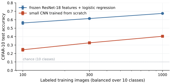
Figure 6.4. CIFAR-10 test accuracy on 2,000 test images as a function of the number of labeled training images, balanced over the ten classes and drawn from a pool of 1000 labeled images, averaged over three seeds with error bars showing the standard deviation across seeds. At 1000 images every seed uses the whole pool, so the seeds differ only in image order and network initialization. Blue, a frozen ResNet-18 feature extractor followed by logistic regression; red, a small convolutional network trained from scratch. The dotted line marks the accuracy of guessing uniformly among ten classes. Produced by Lab 6a.
Show the answer
With only 200 labeled images, freezing the pretrained layers is the safer choice. Fine-tuning adjusts a large number of parameters using very little data, which tends to overfit, and Yosinski et al. (2014) note that for this reason transferred features are often left frozen when the target dataset is small and the number of transferred parameters is large. Fine-tuning becomes worthwhile when more labeled images are available or when only a few top layers are unfrozen.
Security applications
Two security applications of image classification bear on this lesson. The first represents a program as an image. Nataraj et al. (2011) read a malware binary as a sequence of bytes, arranged it as a grayscale image, and computed texture features (GIST) classified by a k-nearest-neighbor rule. On a dataset of 9,458 samples from 25 families they reported about 98% classification accuracy, without disassembling or executing the binary, and noted some resilience to section encryption. The method assigns samples to known families from the visual texture of their byte layout. The result concerns family classification on that dataset and does not show that byte-image methods detect novel malware. A convolutional network can learn texture features of this kind directly from the byte images in place of the hand-designed GIST features.
The second use detects synthetic media. A convolutional classifier can be trained to separate real photographs from images produced by a generator. Wang et al. (2020) trained such a classifier, using a ResNet-50 backbone, on images from one generator (ProGAN) and found that, with suitable data augmentation, it generalized to images from other convolutional generators, which suggests that those generators share systematic artifacts. ResNet-50 is one common choice of backbone among several, and other detectors use different designs. For example, Ojha et al. (2023) report better generalization to unseen generators by classifying in the feature space of a large vision-language model (a CLIP vision transformer) rather than training a convolutional network end to end. Unit 9 returns to synthetic media and to why detectors degrade on generators they have not seen. The image-classification machinery of this lesson is one ingredient of such detectors.
What the lab shows
Lab 6a
A convolutional network and transfer learning
Open in ColabRead with outputsNotebook on GitHubAbout 3 minutes to run on a laptop CPU
In Lab 6a you train the small MNIST network whose parameters Figure 6.2 breaks down, reaching 96.7% accuracy on 2,000 held-out test images after training on a 6,000-image subset, and you inspect its filters and feature maps. You then compare frozen ResNet-18 features against a from-scratch network on CIFAR-10 and reproduce the curve of Figure 6.4, seeing the pretrained features win by the largest margin when labels are fewest.
Summary
A convolutional layer applies a shared local filter at every position, defined by equation \eqref{eq:conv}, with an output size given by equation \eqref{eq:outsize} and a parameter count that does not grow with the input size. In the lab network the convolutional layers hold a few percent of the parameters and the first fully connected layer holds most of them. A stride-1 convolution is translation equivariant away from the input border, but a full network is only approximately invariant to shifts, so transformations that matter must be tested rather than assumed. Stacked layers learn a hierarchy from edges to class-specific structure, and those lower-layer features transfer to new tasks, which lets a frozen pretrained extractor outperform a from-scratch network when labels are scarce. In security, image classification appears in malware byte-image classification and in detectors for synthetic media, each with the scope and limits that the original studies report.
References
- Azulay, A., and Weiss, Y. (2019). Why do deep convolutional networks generalize so poorly to small image transformations?. Journal of Machine Learning Research, 20(184), 1-25. https://jmlr.org/papers/v20/19-519.html
- He, K., Zhang, X., Ren, S., and Sun, J. (2016). Deep residual learning for image recognition. 2016 IEEE Conference on Computer Vision and Pattern Recognition (CVPR), 770-778. https://doi.org/10.1109/CVPR.2016.90
- Krizhevsky, A. (2009). Learning multiple layers of features from tiny images. University of Toronto. Technical report. https://www.cs.toronto.edu/~kriz/learning-features-2009-TR.pdf
- LeCun, Y., Bottou, L., Bengio, Y., and Haffner, P. (1998). Gradient-based learning applied to document recognition. Proceedings of the IEEE, 86(11), 2278-2324. https://doi.org/10.1109/5.726791
- Nataraj, L., Karthikeyan, S., Jacob, G., and Manjunath, B. S. (2011). Malware images: Visualization and automatic classification. Proceedings of the 8th International Symposium on Visualization for Cyber Security (VizSec), 1-7. https://doi.org/10.1145/2016904.2016908
- Ojha, U., Li, Y., and Lee, Y. J. (2023). Towards universal fake image detectors that generalize across generative models. 2023 IEEE/CVF Conference on Computer Vision and Pattern Recognition (CVPR), 24480-24489. https://doi.org/10.1109/CVPR52729.2023.02345
- Wang, S.-Y., Wang, O., Zhang, R., Owens, A., and Efros, A. A. (2020). CNN-generated images are surprisingly easy to spot ... for now. 2020 IEEE/CVF Conference on Computer Vision and Pattern Recognition (CVPR), 8692-8701. https://doi.org/10.1109/CVPR42600.2020.00872
- Yosinski, J., Clune, J., Bengio, Y., and Lipson, H. (2014). How transferable are features in deep neural networks?. Advances in Neural Information Processing Systems, 27. https://proceedings.neurips.cc/paper_files/paper/2014/hash/532a2f85b6977104bc93f8580abbb330-Abstract.html
- Zeiler, M. D., and Fergus, R. (2014). Visualizing and understanding convolutional networks. Computer Vision, ECCV 2014, Lecture Notes in Computer Science 8689, 818-833. https://doi.org/10.1007/978-3-319-10590-1_53