Unit 7 · Lesson 7.2
Gradient attacks, from FGSM to PGD
An adversarial example is an input that a model misclassifies but that a person would judge essentially unchanged, or in a security setting one that still performs its malicious function. Biggio et al. (2013) computed such examples by gradient descent against a PDF malware detector and a handwritten-digit classifier, and Szegedy et al. (2014) found the same brittleness in deep image networks. The striking fact is how little change is needed, and that the change can be computed directly from the model's gradient. This lesson develops the gradient attacks used throughout the field, from the single-step fast gradient sign method to projected gradient descent, with a worked example you can check by hand, and then explains why the image notion of an imperceptible perturbation does not carry over to security, where an attack must preserve function.
The gradient the attacker uses
Training a model computes the gradient of the loss with respect to the parameters and steps the parameters to lower the loss. An attack computes the gradient of the loss with respect to the input and steps the input to raise the loss, holding the parameters fixed. These are different gradients of the same loss. One points in parameter space and the other in input space. An attack therefore performs gradient ascent on the loss in input space, which is a different computation from running the training step in reverse.
Write \(L(x, y)\) for the loss of the model on input \(x\) with true label \(y\), and \(\nabla_x L(x, y)\) for its gradient with respect to the input. An untargeted attack seeks a small change to \(x\) that increases \(L\), which tends to change the predicted label.
The fast gradient sign method
Goodfellow et al. (2015) proposed taking a single step of a fixed size in the direction that increases the loss fastest under an \(L_\infty\) bound. The fast gradient sign method (FGSM) is
where \(\varepsilon\) is the budget, \(\mathrm{sign}\) takes the sign of each component, and \(\mathrm{clip}\) returns the result to the valid input range. Before clipping, the sign moves every component with a nonzero gradient by exactly \(\varepsilon\), so the perturbation has \(L_\infty\) norm \(\varepsilon\), the largest change allowed to any single feature; clipping can only shrink a component. The method is called fast because it needs one gradient evaluation.
Why a tiny perturbation suffices is explained by linearity. Goodfellow et al. (2015) argue that modern networks behave linearly enough over the relevant scale that a perturbation aligned with the weights adds up across many dimensions. For a linear model with weights \(w\), the change in the logit from a perturbation \(\eta\) is \(w^\top \eta\, \); choosing \(\eta = \varepsilon\, \mathrm{sign}(w)\) makes this \(\varepsilon \sum_i |w_i| = \varepsilon \|w\|_1\), which grows with the number of dimensions even though each component moves by only \(\varepsilon\). High-dimensional inputs therefore admit large changes to the output from small changes to each feature.
A logistic model makes the arithmetic concrete. Take weights \(w = (2, -1)\), bias \(b = 0\), input \(x = (0.5, 0.2)\) with each feature valid in the interval from 0 to 1, and true label \(y = 1\). The logit is \(z = w^\top x = 0.8\), and the predicted probability is \(p = \sigma(0.8) = 0.690\), where \(\sigma(z) = 1/(1 + e^{-z})\) is the logistic sigmoid. For logistic loss the input gradient is \(\nabla_x L = (p - y)\, w\), which here equals \((0.690 - 1)(2, -1)\), that is \((-0.62, 0.31)\), whose sign is \((-1, +1)\). With \(\varepsilon = 0.1\), equation \eqref{eq:fgsm} gives \(x_{\mathrm{adv}} = (0.4, 0.3)\). The new logit is \(z_{\mathrm{adv}} = w^\top x_{\mathrm{adv}} = 0.5\) and \(p_{\mathrm{adv}} = \sigma(0.5) = 0.622\), so the confidence in the true class has fallen. The logit dropped by exactly \(\varepsilon \|w\|_1 = 0.1 \times (2 + 1) = 0.3\), matching the linear analysis. Figure 7.4 plots the two points on the sigmoid.
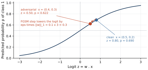
Figure 7.4. The worked FGSM example on a logistic model with weights (2, -1). The clean input has logit 0.80 and probability 0.690 for class 1; one FGSM step with budget 0.1 moves it to logit 0.50 and probability 0.622. The logit falls by eps times the L1 norm of the weights, 0.1 times 3 = 0.3. From the worked example, recomputed in Python.
Show the answer
The sign of the gradient is unchanged, \((-1, +1)\), so the first coordinate falls by 0.3 and the second rises by 0.3, giving \(x_{\mathrm{adv}} = (0.2, 0.5)\). The new logit is \(z_{\mathrm{adv}} = 2 \times 0.2 - 1 \times 0.5\), which equals \(-0.1\) and is now on the other side of the decision boundary at zero. The logit dropped by \(\varepsilon \|w\|_1 = 0.3 \times 3 = 0.9\), from 0.8 to -0.1.
From one step to many: BIM and PGD
A single step of fixed size overshoots in some directions and undershoots in others. Taking several smaller steps, re-evaluating the gradient at each, finds stronger adversarial examples within the same budget. Kurakin et al. (2017) proposed the basic iterative method (also called I-FGSM), which applies FGSM in small steps and clips each intermediate result back into the \(\varepsilon\)-ball around the original input.
Madry et al. (2018) formalized this as projected gradient descent (PGD) and framed robustness as a saddle-point problem in which the defender chooses the model parameters to minimize the expected loss and the attacker chooses a perturbation within the allowed set to maximize it. PGD performs gradient ascent on the loss and projects back onto the feasible set after each step,
where \(\alpha\) is the step size, \(\Pi_{\mathcal{S}}\) projects onto the feasible set \(\mathcal{S}\), which is the intersection of the \(\varepsilon\)-ball around the original input and the valid input range, and the iteration starts from a random point inside the \(\varepsilon\)-ball rather than from \(x\) itself. PGD is more than FGSM applied repeatedly. The random start explores different starting points, and the projection keeps every iterate feasible, so it is a genuine constrained optimization rather than a fixed step taken several times. Running it from several random starts, called restarts, and keeping the strongest result makes it a strong attack, and Madry et al. (2018) give evidence that it is the strongest attack that uses only first-order (gradient) information about the network. Figure 7.5 shows one FGSM step and a PGD path with a projection.
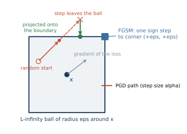
Figure 7.5. The L-infinity ball of radius eps around an input x. FGSM takes one sign step to a corner of the ball (blue). PGD starts at a random point, takes small gradient-sign steps, and when a step leaves the ball projects it back onto the boundary (green), keeping every iterate feasible. Drawn as a schematic.
Show the answer
The feasible set is the box with first coordinate in \([0.4, 0.6]\) and second in \([0.1, 0.3]\), which lies inside the valid range, so the projection \(\Pi_{\mathcal{S}}\) clips each coordinate to its interval. The start is feasible, since it differs from \(x\) by 0.05 and 0.07, and its logit is \(2 \times 0.45 - 0.27 = 0.63\). The gradient \((p - y)\, w\) has sign \((-1, +1)\) because \(p < 1\). The first step gives \((0.41, 0.31)\), and projection clips the second coordinate, so \(x^{(1)} = (0.41, 0.30)\) with logit 0.52. The second step gives \((0.37, 0.34)\), which projects to \(x^{(2)} = (0.40, 0.30)\) with logit 0.50 and probability 0.622. Every later step leaves the box in the same direction and is projected back to the same corner, so the iteration stays at \((0.4, 0.3)\), the FGSM point. For a linear model the sign of the input gradient is the same everywhere, so the best \(L_\infty\) perturbation is the corner that FGSM reaches in one step. PGD finds stronger examples only when the loss is nonlinear and the gradient sign changes along the path.
The Carlini-Wagner attack (Carlini and Wagner, 2017) takes a different route. Instead of maximizing the loss within a fixed budget, it minimizes the size of the perturbation needed to cause a misclassification, using a carefully chosen objective and a continuous optimizer. In the authors' experiments it was about ten times slower than the iterative gradient sign method, and its \(L_0\) and \(L_2\) versions found adversarial examples with 2 to 10 times lower distortion than the best previously published attacks. It is a common choice when the question is how little change is needed rather than how much damage a fixed budget does.
Epsilon conventions
A budget \(\varepsilon\) is meaningless without a norm and an input scale. Under the \(L_\infty\) norm, with pixel values scaled to the interval from 0 to 1, the conventional budgets are \(0.3\) for MNIST and \(8/255 \approx 0.031\) for CIFAR-10, the values used by Madry et al. (2018), who state the CIFAR-10 budget as 8 on the 0 to 255 pixel scale. The two budgets differ by a factor of almost ten because the images differ. On MNIST a change of 0.3 per pixel leaves digits recognizable to a person, while on CIFAR-10 color photographs the same change would be glaring, so a much smaller budget is used. A budget must fit the scale of the data; a value chosen for one dataset or one input representation does not transfer to another, and quoting \(\varepsilon\) without the norm and scale is a frequent source of confusion.
Why "imperceptible" does not transfer to security
For images the constraint is perceptual, since the perturbation should be too small for a person to notice. That constraint does not apply to most security data. A malware file is not viewed, so there is nothing to keep imperceptible; a perturbation that is small in some feature norm may still break the program. The real constraint is functional. An adversarial malware sample must still run and perform its malicious behavior, and an adversarial network flow must still carry out the attack it encodes. Describing such perturbations as invisible or imperceptible misstates the constraint, which is on function, not perception.
This is the problem-space view of Lesson 7.1. Pierazzi et al. (2020) formalize problem-space evasion as subject to constraints on the available transformations, the semantics that must be preserved, robustness to preprocessing, and plausibility, and they show that a feature-space perturbation does not always correspond to a realizable object. Grosse et al. (2017) attack a malware detector under one such constraint, preserved semantics, modifying an Android application by only adding entries that do not change its behavior, so that the sample remains functional. A feature-space attack offers no such guarantee. Apruzzese et al. (2023) argue from real-world evidence that actual attackers use simple tactics to subvert machine-learning systems. In one of their three case studies, phishing pages confused a commercial detector through manipulations such as cropping, masking or blurring the logo, which need no gradient computations. They argue for threat models that are precise about capability and cost. This is a reason to model capability realistically rather than assume a gradient-based worst case everywhere. Lab 7b implements a constrained flow attack and measures how much the constraints reduce the evasion rate.
What the labs show
Lab 7a
FGSM and PGD against an image classifier
Open in ColabRead with outputsNotebook on GitHubAbout 2 minutes to run on a laptop CPU
In Lab 7a you implement FGSM and PGD by hand against a small MNIST classifier, with random start, step size, projection and clipping, and draw robustness curves. Figure 7.6 shows accuracy falling as the budget grows, with PGD at or below FGSM everywhere, and Figure 7.7 shows example digits and their adversarial versions. At \(\varepsilon = 0.1\) the classifier's accuracy falls to 61.9% under PGD, and at \(\varepsilon = 0.3\) it reaches 0.0%, the sanity check that Lesson 7.3 explains.
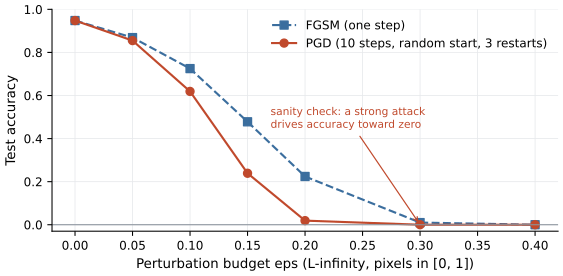
Figure 7.6. Test accuracy of the lab's MNIST classifier on 1,000 test digits under FGSM (one step) and PGD (10 steps, random start, 3 restarts) as the L-infinity budget grows from 0 to 0.4, with pixels in the interval from 0 to 1. PGD is at or below FGSM at every budget, and a strong attack drives accuracy toward zero. Produced by Lab 7a.
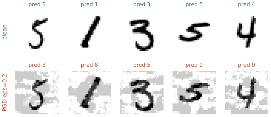
Figure 7.7. Top, clean MNIST digits with the classifier's correct predictions. Bottom, the same digits after a PGD attack with budget 0.2, with the classifier's now-incorrect predictions. The perturbation is visible at this budget. Produced by Lab 7a.
Lab 7b
Evading a network detector under realistic constraints
Open in ColabRead with outputsNotebook on GitHubAbout 1 minute to run on a laptop CPU
Lab 7b attacks a network-flow detector first with a feature-space attack bounded only by an \(L_\infty\) budget and then under problem-space-style constraints, and reports how far the evasion rate falls when the constraints are imposed. Lesson 7.3 and that lab develop the point that such a feature-space evasion rate overstates the real risk.
Summary
Gradient attacks compute adversarial examples, inputs crafted to be misclassified, from the gradient of the loss with respect to the input, which is a different gradient from the one training uses and is ascended, not reversed. FGSM takes one \(L_\infty\) step of size \(\varepsilon\) in the sign of that gradient, equation \eqref{eq:fgsm}, and the worked logistic example shows the logit falling by \(\varepsilon \|w\|_1\). PGD, equation \eqref{eq:pgd}, performs projected gradient ascent from a random start and is a strong, standard attack, distinct from FGSM repeated. Budgets are tied to a norm and an input scale, with \(0.3\) for MNIST and \(8/255\) for CIFAR-10 under \(L_\infty\). In security the binding constraint is that the modified object still functions, which is the problem-space setting, and the attacks documented in practice mostly use simple manipulations that need no gradients.
References
- Apruzzese, G., Anderson, H. S., Dambra, S., Freeman, D., Pierazzi, F., and Roundy, K. (2023). 'Real attackers don't compute gradients': Bridging the gap between adversarial ML research and practice. 2023 IEEE Conference on Secure and Trustworthy Machine Learning (SaTML), 339-364. https://doi.org/10.1109/SaTML54575.2023.00031
- Biggio, B., Corona, I., Maiorca, D., Nelson, B., Šrndić, N., Laskov, P., Giacinto, G., and Roli, F. (2013). Evasion attacks against machine learning at test time. Machine Learning and Knowledge Discovery in Databases (ECML PKDD), Lecture Notes in Computer Science 8190, 387-402. https://doi.org/10.1007/978-3-642-40994-3_25
- Carlini, N., and Wagner, D. (2017). Towards evaluating the robustness of neural networks. 2017 IEEE Symposium on Security and Privacy (SP), 39-57. https://doi.org/10.1109/SP.2017.49
- Goodfellow, I. J., Shlens, J., and Szegedy, C. (2015). Explaining and harnessing adversarial examples. International Conference on Learning Representations (ICLR). arXiv preprint arXiv:1412.6572. https://arxiv.org/abs/1412.6572
- Grosse, K., Papernot, N., Manoharan, P., Backes, M., and McDaniel, P. (2017). Adversarial examples for malware detection. Computer Security, ESORICS 2017, Lecture Notes in Computer Science 10493, 62-79. https://doi.org/10.1007/978-3-319-66399-9_4
- Kurakin, A., Goodfellow, I. J., and Bengio, S. (2017). Adversarial examples in the physical world. International Conference on Learning Representations (ICLR) Workshop Track. arXiv preprint arXiv:1607.02533. https://arxiv.org/abs/1607.02533
- Madry, A., Makelov, A., Schmidt, L., Tsipras, D., and Vladu, A. (2018). Towards deep learning models resistant to adversarial attacks. International Conference on Learning Representations (ICLR). arXiv preprint arXiv:1706.06083. https://arxiv.org/abs/1706.06083
- Pierazzi, F., Pendlebury, F., Cortellazzi, J., and Cavallaro, L. (2020). Intriguing properties of adversarial ML attacks in the problem space. 2020 IEEE Symposium on Security and Privacy (SP), 1332-1349. https://doi.org/10.1109/SP40000.2020.00073
- Szegedy, C., Zaremba, W., Sutskever, I., Bruna, J., Erhan, D., Goodfellow, I., and Fergus, R. (2014). Intriguing properties of neural networks. International Conference on Learning Representations (ICLR). arXiv preprint arXiv:1312.6199. https://arxiv.org/abs/1312.6199