Working Notes on Large Language Models
8. Evaluation: benchmarks and LLM-as-a-judge
Every chapter so far has ended with a number, and this one is about where those numbers come from and how they lie. It runs three evaluations of three different kinds. A harness that scores the chapter 4, 5 and 6 models on the same prompts with the same rule, which is the honest kind and the kind that found something the earlier chapters missed. A demonstration of contamination, where a model is scored on text it trained on. And a language model used as a judge of other models' answers, tested for the bias that judges are most often caught with, which it has in the purest form I have seen.
The numbers come from 08-evaluation.ipynb as executed: 343 seconds on the laptop described in chapter 1.
8.1 A harness
An evaluation harness is a fixed set of prompts, a fixed decoding rule, and a fixed scoring rule, applied identically to every model. The fixed parts are the point. Change any of them between models and you are no longer comparing models.
Here: 100 held-out word lists per task, the four tasks of chapters 4 to 6, greedy decoding, exact match after stripping a trailing full stop, and a last column for how often the answer ends with one, averaged over the four tasks. The same random seed for every model, so every model sees the same 400 prompts.
| reverse | repeat | last | reverse and repeat | ends with full stop | |
|---|---|---|---|---|---|
| chapter 3 (base) | 0% | 0% | 0% | 0% | 1% |
| chapter 4 (SFT) | 64% | 76% | 100% | 0% | 0% |
| chapter 5 (DPO) | 61% | 76% | 100% | 0% | 100% |
| chapter 6 (GRPO) | 38% | 20% | 99% | 27% | 0% |
Figure 8.1 shows the same numbers as a grid.
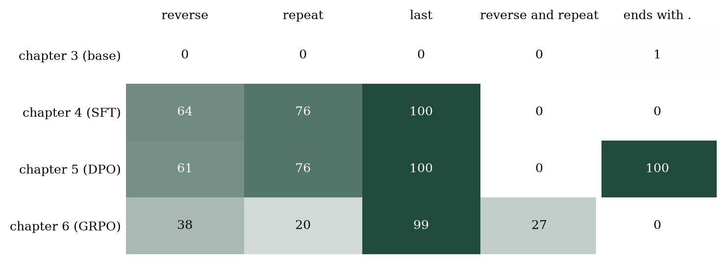
Figure 8.1. Exact match in percent on 100 held-out lists per task, for each model, with the last column the percentage of answers ending in a full stop over all four tasks. Darker is higher.
Thirty-five seconds to produce, and it says three things the chapters did not.
The DPO model kept repeat and last exactly where the chapter 4 model had them and dropped three points on reverse, a small change on 100 prompts, while ending every one of its 400 answers with a full stop. Chapter 5 measured 78% correct on a mixed sample; the per-task breakdown is cleaner.
The GRPO model learned the composed task (27% on reverse and repeat, from 0%; chapter 6 measured 32% on a different 100 lists) and lost most of what it had on the tasks it was not trained on: repeat fell from 76% to 20%, and reverse from 64% to 38%. Chapter 6 did not measure that, because chapter 6 measured the task it was training. Three hundred steps of reinforcement on one instruction, with a KL penalty against the chapter 4 model that was evidently not strong enough, eroded skills that no prompt in the RL batch ever asked for. The chapter 6 KL of about 4 to 5 nats per token was the warning, and this table is what it was warning about. The same forgetting happened in chapter 4 (the book) and it happens, at scale, every time a model is tuned on a narrow objective; the only defence is a harness that keeps scoring the things you are not training.
The reverse column is the one to be modest about. 64%, 61%, 38%: the SFT and DPO models are close to the same model on this task, and GRPO cost it 26 points. Any of these could be quoted as "the model reverses lists", and none of them is a model you would rely on to.
8.2 Contamination
Take the chapter 3 model, the one kept at its best held-out loss, and train it for another 600 steps on the training text, 247 seconds. Chapter 3 showed that this turns it into a copy of the book. Now build two benchmarks: 20 passages from the training text and 20 from the held-out text, scored by next-token accuracy.
| training passages | held-out passages | |
|---|---|---|
| chapter 3 model | 29.9% | 22.1% |
| same model, 600 more steps | 87.6% | 18.6% |
On the first benchmark the extra training looks like the best thing that ever happened to this model: 29.9% to 87.6%. On the second it made the model worse. The first benchmark is contaminated; it measures recall of the training set and nothing else. Even the original model shows the gap, 29.9% against 22.1%, because it saw those passages too, at a lower dose. Figure 8.2 shows the four numbers side by side.
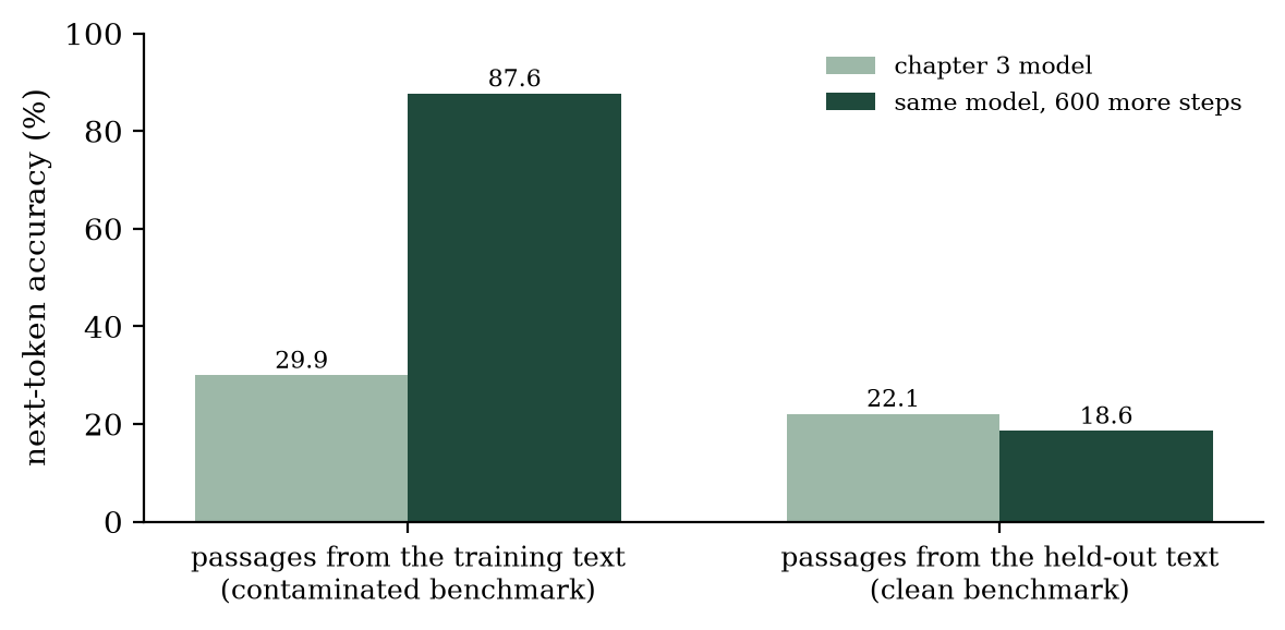
Figure 8.2. Next-token accuracy in percent on 20 passages of 128 tokens from the training text (a contaminated benchmark) and 20 from the held-out text (a clean one), for the chapter 3 model and for the same model after 600 more steps on the training text.
This is the whole of the contamination problem at a scale where you can see both numbers. For a model trained on a crawl of the internet, the benchmark's test questions are somewhere in that crawl with a probability that rises every year the benchmark is public, nobody has the held-out column, and the model's score on the public column goes up for reasons that have nothing to do with ability. The defences are the ones this notebook uses: a split made before training, a benchmark written after the training data was collected, or a benchmark that can be regenerated (chapter 4's word lists are one; a new list is as fresh as a new random seed).
8.3 A language model as a judge
For most outputs there is no exact-match rule. The standard move is to ask a capable model to compare two answers. The question is whether the judge is measuring the answers or something else, and the cheapest test is to show it the same pair twice in the two orders.
Forty pairs of answers to reverse the words, one correct and one with two adjacent words swapped, shown to the chapter 7 model (SmolLM2-360M-Instruct) as Answer A and Answer B with the question "Which answer is correct? Reply with the single letter A or B." The verdict is read from the model's next-token probabilities for A and B rather than sampled, so there is no noise in it. Each pair is shown in both orders. Eighty judgements, 44 seconds. The results are in the table and Figure 8.3.
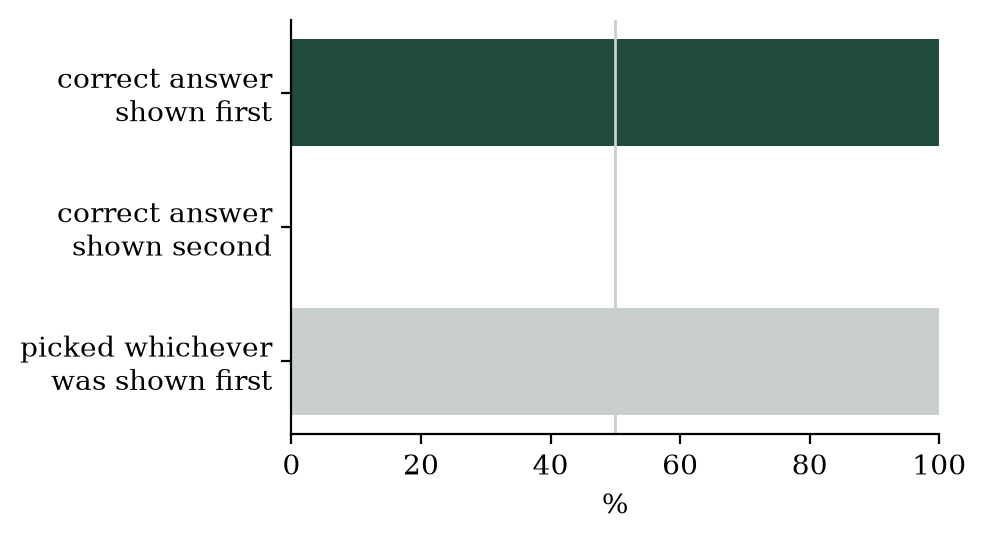
Figure 8.3. The judge's accuracy when the correct answer is shown first, when it is shown second, and how often it picked whichever answer was listed first, over 40 pairs shown in both orders; the vertical line marks 50%, the accuracy of a coin flip.
| accuracy when the correct answer is A | 100% |
| accuracy when the correct answer is B | 0% |
| overall accuracy | 50% |
| same verdict in both orders | 0% |
| chose the first-listed answer | 100% |
The judge picked A eighty times out of eighty. Its "accuracy" of 50% is the accuracy of a rule that says A, and its agreement with itself across orders is zero. Had the pairs been shown in one order only, with the correct answer first, the notebook would have reported a perfect judge.
A 362-million-parameter model is an extreme case, but the bias it shows in pure form has also been measured, in weaker form, in much larger judges. In a position-bias test built from pairs of very similar answers, Zheng et al. (2023) found that GPT-4 gave the same verdict in both orders in only 65% of cases. Position bias, length bias (preferring the longer answer) and self-preference (preferring its own answers) are the three to test for. The same study found clear position bias, found length bias strongly in two judges and weakly in GPT-4, and could not settle the third, which is a reason to test for it rather than assume an answer. The test is the same for all of them: change the thing that should not matter and see whether the verdict changes. Exercise 2 adds the standard mitigation, judging in both orders and counting only agreements, and asks what it costs in coverage.
8.4 Putting the three together
The harness is the thing to build first and keep running: fixed prompts, fixed rules, every model, including the ones you are not currently working on. The contamination check is a question to ask of every benchmark you did not generate yourself: did the model see this? The judge is a tool to use only after you have measured the judge, in both orders, on pairs where you know the answer.
The two biggest surprises in these notes, the forgetting in chapters 4 and 8 and the collapse in chapter 5, were both found by the first kind. A training loss never found anything.
Where this goes wrong
One order. A judge shown pairs in one order is a judge whose bias you have decided not to see.
One benchmark. A single number on a single benchmark cannot distinguish a better model from a contaminated one. Two benchmarks with different exposure can.
Measuring only the target. Chapter 6 reported 32% on the task it trained and did not report the fall from 76% to 20% on a task it damaged. The harness exists so that the second number is never optional.
Exercises
- Run the judge with the letters swapped for
1and2, then forfirstandsecond. Does the bias follow the position or the label? - Show the judge both orders and accept a verdict only when they agree. Report accuracy on the pairs it is sure about and the fraction it refuses. This is the standard fix; what does it cost?
- Make the wrong answers subtler: swap the two middle words of a five-word list only. Rerun. Where does judge accuracy fall to chance?
- Build a harness for the chapter 3 model's held-out loss that reports a 95% confidence interval from bootstrap resampling of the 20 batches. How many batches do you need before two models 0.1 nats apart can be told apart?
- The contamination section trained for 600 extra steps. Find the smallest number of extra steps at which the training-passage benchmark overstates the held-out one by 10 percentage points. What does that say about how much contamination it takes?
Notebook for this chapter: 08-evaluation.ipynb, 343 seconds in total. It reads the chapter 3 to 6 checkpoints from the repository and the chapter 7 model from the Hugging Face cache.
Further reading
- Lianmin Zheng, Wei-Lin Chiang, Ying Sheng, et al. 2023. Judging LLM-as-a-judge with MT-Bench and Chatbot Arena. Advances in Neural Information Processing Systems 36 (NeurIPS 2023), Datasets and Benchmarks Track, 46595-46623. arXiv:2306.05685.