5. Tuning on preferences: RLHF, PPO and DPO

Dr. Ali Al Bataineh, Higher Colleges of Technology, United Arab Emirates

Chapter 4 taught the model what to answer. This chapter changes how it answers, using nothing but pairs: for each prompt, one answer that is preferred and one that is not. No example of the preferred behaviour is ever presented as a target to copy. That is the shape of the data behind the manners of most chat models, and this chapter runs the two standard ways of learning from it on the chapter 4 model, with a preference simple enough to count: a good answer is correct and ends with a full stop.

The first DPO run I did went wrong, in a way that is well documented and still catches people. The chapter keeps it, next to the run that works, because the difference between them is the content of the chapter. All numbers come from 05-preferences.ipynb as executed: 209 seconds on the laptop described in chapter 1.

5.1 Where the preference lives

The chapter 4 model answers the three word-list instructions correctly 80% of the time and never ends with a full stop, since nothing in its training data had one. Given a correct answer with a full stop and a corrupted one without, it assigns more probability to the correct one on only 37% of pairs. The full stop is an unfamiliar token at that position and costs more probability than the corruption does.

That 37% is the baseline. A method that learns from preferences should move it toward 100%, and it should do so without wrecking the 80%.

5.2 The pairs

4,000 training pairs and 300 held-out pairs. The chosen answer is the correct one with a full stop. The rejected answer is a corruption without one: for reverse, two adjacent words swapped; for repeat, one copy too many; for last, the first word instead of the last.

Instruction: repeat the words
Words: sure will another course
Answer:
  chosen    sure will another course sure will another course.
  rejected  sure will another course sure will another course sure will another course

Notice how much the two answers share. In the repeat example the rejected answer contains the chosen one, minus the full stop. That overlap is realistic, since real preference pairs are usually two decent answers that differ in a detail, and it is also the cause of what goes wrong in section 5.4.

5.3 A reward model

The first half of RLHF is a model that scores answers. Here it is a copy of the chapter 4 model with the vocabulary head replaced by a single number read from the last token, trained for 300 steps on the pairs with the Bradley-Terry loss,

$$ \mathcal{L} = -\log \sigma\big(r_\theta(x, y_w) - r_\theta(x, y_l)\big), $$

which only asks that the chosen answer score higher than the rejected one; the scores have no units. In 34 seconds it reaches a loss of 0.002 and ranks 99.7% of held-out pairs correctly. The task is easy for a model that already knows the right answers, since the corruptions are visible.

In full RLHF (Ouyang et al., 2022) this reward model would now score samples from the policy, and a PPO loop (Schulman et al., 2017) would push the policy toward higher scores while a KL term holds it near the starting point. That machinery has four models in memory (policy, reference, reward, value) and a sampling loop, and it is the reason chapter 6 exists as a separate chapter. DPO (Rafailov et al., 2023) is the observation that, for this particular objective, the reward model and the sampling loop can be dropped.

5.4 Direct preference optimisation

The policy starts as a copy of the chapter 4 model; another frozen copy is the reference. For each pair,

$$ \mathcal{L}_{\text{DPO}} = -\log \sigma\!\left(\beta \left[ \log\frac{\pi_\theta(y_w \mid x)}{\pi_{\text{ref}}(y_w \mid x)} - \log\frac{\pi_\theta(y_l \mid x)}{\pi_{\text{ref}}(y_l \mid x)} \right]\right), $$

where $\pi(y \mid x)$ is the probability of the whole answer, the sum of its token log-probabilities. The bracket is the margin between how much the policy has raised the chosen answer and how much it has raised the rejected one, both relative to the reference; the loss wants it large and positive. $\beta$ is 0.1. Three runs, 300 steps of 16 pairs each, between 48 and 59 seconds apiece. The table gives the results and Figure 5.1 the training curves.

	prefers chosen (held-out pairs)	correct answers	ends with full stop	log p(chosen), policy minus reference
chapter 4 model	37%	80%	0%	0
DPO, lr $10^{-4}$	100%	38%	48%	-9.2 nats
DPO, lr $10^{-5}$	100%	5%	0%	+17.2 nats
DPO, lr $10^{-4}$, plus SFT term	100%	78%	100%	+46.0 nats

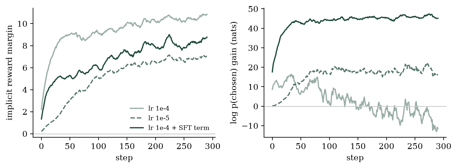
Implicit reward margin and chosen-answer log-probability during the three DPO runs

Figure 5.1. Left: the margin inside the sigmoid, 10-step mean. Right: the policy's log-probability of chosen answers relative to the reference. The run without the SFT term at the higher learning rate drives its margin up while the chosen answers themselves become less likely.

The first run learns the preference perfectly, by the measure DPO optimises: 100% of held-out pairs ranked right, loss 0.000. And the model it produces is broken. Correct answers fall from 80% to 38%, the full stop appears 48% of the time, and the samples are things like came from. with came. The last column says why. The log-probability of the chosen answers went down by 9.2 nats. DPO's loss only constrains the gap between chosen and rejected; the cheapest way to open a gap between two answers that share most of their tokens is to push the rejected one down hard, and because they share tokens, the chosen one goes down with it. The margin is satisfied, the policy has moved its mass somewhere else entirely, and generation samples from wherever that is. Razin et al. (2025) call this likelihood displacement. They link it to pairs whose chosen and rejected answers have similar hidden representations inside the model, a measure they find more predictive than token-level overlap, so the shared-token account above is an intuition rather than the whole mechanism. The signature is exactly the one in the table: pair accuracy near 100%, sample quality collapsed, chosen log-probability negative.

The second run, ten times gentler, avoids that signature and is worse. The chosen log-probability goes up, by 17.2 nats, and pair accuracy is 100%, yet the full stop never appears and correct answers fall to 5%. Raising the probability of whole chosen answers relative to the reference is not the same as making them the answers the model gives. Greedy decoding follows the most likely next token at each step, and DPO moved probability in ways that neither the pair accuracy nor the chosen log-probability shows. Turning the learning rate down is not a fix.

The third run adds a common repair, of the kind Pang et al. (2024) found crucial in their own setting: a supervised term on the chosen answer, the mean negative log-likelihood per chosen token, weighted 0.5, added to the DPO loss. Now the loss cannot be satisfied by pushing both answers down, because the chosen one is being pulled up directly. Result: 100% on pairs, 78% correct answers, a full stop on 100% of them, chosen log-probability up 46.0 nats. One of the three samples printed in the notebook is the chapter 4 model's answer with a full stop added. In another, came from tried with., two words that the chapter 4 model had in the right order are swapped, and the third changes the last word of an answer that was already wrong. That is what a two-point drop in accuracy looks like up close. This is the model saved to checkpoints/05-dpo.pt.

loss = -F.logsigmoid(margin).mean()
if sft_weight:   # keep the chosen answers likely
    lengths = torch.tensor([len(c) for c in C], dtype=torch.float)
    loss = loss + sft_weight * (-(pol_w / lengths)).mean()

5.5 What this says about the method

DPO is exact: it optimises the same objective as RLHF with a particular reward model, without training that model. The exactness is about the objective, not about what gradient descent on it does from a given starting point with a given learning rate. The objective is satisfied by any policy that separates chosen from rejected, including policies that have abandoned both. Something has to anchor the policy to answers worth giving, and in the third run that is the SFT term. The second run is a warning that a lower learning rate on its own is not an anchor; exercise 1 tries $\beta$ instead. Whatever the anchor, the pair-accuracy number that the DPO loss reports is never the number to trust. Figure 5.2 makes the point with all four models.

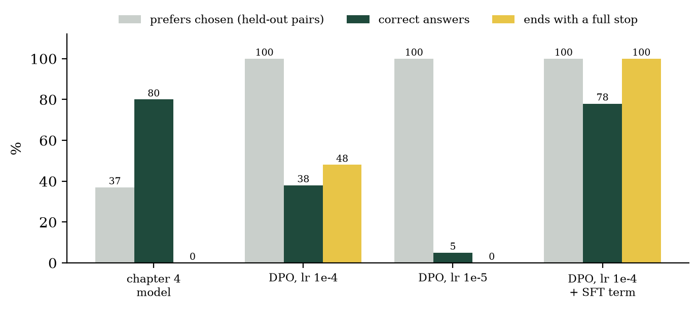
Pair accuracy, correct answers and full-stop rate for the chapter 4 model and the three DPO runs

Figure 5.2. For the chapter 4 model and the three DPO runs: how often the model puts more probability on the chosen answer of a held-out pair (the quantity DPO trains), how often its greedy answer to a held-out prompt is correct, and how often that answer ends with a full stop. 300 held-out pairs and 100 held-out prompts, in percent. Sample from the model and look.

Where this goes wrong

Reading pair accuracy as success. All three runs score 100% on pairs. Two of them are unusable. Pair accuracy is the training objective; it is not the thing you wanted.

Pairs that are too similar. When chosen and rejected share most tokens, DPO's gradient on the shared tokens nearly cancels and what remains pushes the rest around. This is the regime of real preference data, so it is not avoidable, only manageable.

Not watching the chosen log-probability. It is one line to compute, it is in the notebook's log, and in the first run it told the story before the samples did. If it goes negative, stop. The second run shows that the converse does not hold. A positive value is no guarantee, and only the samples are.

Exercises

Set $\beta$ to 0.01 and to 1.0 with the SFT term and retrain. Report the full-stop rate, the accuracy, and the mean KL between policy and reference on held-out prompts. What does $\beta$ trade?
Make the rejected answers correct answers without a full stop, so the only difference in each pair is the full stop. Does DPO without the SFT term still collapse, and does the SFT term still help?
Use the reward model as a filter: generate 8 answers per prompt from the chapter 4 model at temperature 1.0, keep the highest-scoring one, and measure accuracy and full-stop rate. This is best-of-n sampling. Compare with DPO at equal compute.
The reward model reads a score from the last token. Read it from the mean of all answer tokens instead and compare held-out ranking accuracy.
Train DPO on pairs from reverse and repeat only. Report the full-stop rate on last. Does the preference transfer to an instruction it was never trained on?

Notebook for this chapter: 05-preferences.ipynb, 209 seconds in total, no downloads. It writes checkpoints/05-dpo.pt, which chapter 8 scores.