1. Attention and the transformer block

Dr. Ali Al Bataineh, Higher Colleges of Technology, United Arab Emirates

This chapter builds the smallest transformer that does something worth looking at. You will write scaled dot-product attention by hand, stack it into a two-block model with 103,244 parameters, and train that model to read a string of letters and write it backwards. Training takes 41 seconds on a laptop CPU. The model is small enough that you can print any tensor inside it, and the attention weights it learns are legible, which is why I start here instead of with a pretrained model you cannot see into.

You need Python, a little NumPy, and enough linear algebra to multiply two matrices and know what a dot product measures. The code is PyTorch, but it is PyTorch used as NumPy with gradients; nothing in it assumes you have seen the library before.

Every number in this chapter comes from one of two notebooks as executed: 01-attention.ipynb, which builds and tests the model, and 01-attention-experiments.ipynb, which retrains it with deliberate faults. Both ran on the laptop used for every chapter of these notes, an Intel Core Ultra 7 155U running Windows 11 and Python 3.12, with PyTorch limited to four CPU threads and no GPU. A faster machine will take less time and should give the same numbers.

1.1 What the block has to do

A language model reads a sequence of tokens and, at every position, predicts the next one. Inside the model each token is a vector, and a transformer block is a function that takes the whole sequence of vectors in and gives a sequence of the same shape back. It has two jobs. Each position has to collect information from the positions before it, because the right next token depends on context. Then each position has to compute something from what it collected. Attention does the collecting. A small feed-forward network does the computing. Everything else in the block is there to keep training stable.

That division of labour is worth holding on to. When a model fails, the question "did it fetch the wrong thing, or do the wrong thing with it?" is usually the first one to ask.

1.2 Attention by example

Suppose the model is reading the cat sat on it and has reached it. To predict what comes next, it would help to know what it refers to. Attention lets the position holding it ask every earlier position a question and collect an answer, weighted by how relevant each position is.

Each token gets three vectors. The query says what this position is looking for. The key says what this position contains. The value is what this position hands over if someone attends to it. The query of the current token is compared with the key of every token it is allowed to see, the comparison scores are turned into weights that sum to one, and the output is the weighted sum of the values.

Here is the arithmetic for it, with 2-dimensional vectors so you can follow it on paper. The query for it is (1, 2). The keys and values of the four earlier tokens are in the table. A score is the dot product of the query with a key, divided by the square root of the dimension, which is 1.41 here.

key token	key vector	value vector	score	weight
the	(0, 0)	(0, 0)	0.00	0.02
cat	(1, 2)	(2, 1)	3.54	0.83
sat	(1, 0)	(0, 1)	0.71	0.05
on	(0, 1)	(1, 0)	1.41	0.10

The weights are the softmax of the four scores: exponentiate each, divide by the sum. it puts 83% of its weight on cat, which is the behaviour you would want from a pronoun. The output for it is the weighted sum of the value vectors, 0.83 × (2, 1) + 0.10 × (1, 0) + 0.05 × (0, 1) + 0.02 × (0, 0). With the rounded weights that is (1.76, 0.88); the notebook keeps full precision and prints (1.75, 0.88). The output is dominated by what cat chose to hand over, with a little of on and sat mixed in.

Notice what the query and key did and did not do. They decided where to look. They had no say in what was fetched; that is the value's job. Keep the two separate in your head, because the plots later in the chapter show only the first half.

1.3 The same thing as an equation

Stack the queries of all positions into a matrix $Q$ with one row per token, and likewise the keys into $K$ and the values into $V$. Then the whole computation, in the form introduced with the transformer by Vaswani et al. (2017), is

$$ \mathrm{Attention}(Q, K, V) = \mathrm{softmax}\!\left(\frac{QK^{\top}}{\sqrt{d_k}}\right) V , $$

where $d_k$ is the dimension of a query or key. $QK^{\top}$ is a square matrix of scores, one row per query and one column per key. The softmax is applied to each row separately, so the weight that query $i$ puts on key $j$ is

$$ w_{ij} = \frac{\exp(s_{ij})}{\sum_{j'} \exp(s_{ij'})}, \qquad s_{ij} = \frac{q_i \cdot k_j}{\sqrt{d_k}} , $$

and row $i$ of the output is $\sum_j w_{ij}\, v_j$. The sum in the denominator runs over keys. That is the detail to remember from this chapter: the softmax normalises over keys, so every row of the weight matrix sums to one.

In code the equation is a dozen lines, and the version below is the one the project uses. It also returns the weights so we can plot them.

def attention(q, k, v, causal=True):
    # q, k, v: (batch, tokens, dim)
    d = q.shape[-1]
    scores = q @ k.transpose(-2, -1) / math.sqrt(d)            # (batch, tokens, tokens)
    if causal:
        T = scores.shape[-1]
        mask = torch.triu(torch.ones(T, T, dtype=torch.bool), diagonal=1)
        scores = scores.masked_fill(mask, float("-inf"))      # no looking ahead
    weights = F.softmax(scores, dim=-1)                       # rows sum to one
    return weights @ v, weights

dim=-1 is the key axis. The last section of the chapter shows what happens when it is the query axis instead.

1.4 Why the square root

Suppose the entries of a query and a key are independent, with mean zero and variance one. Their dot product is a sum of $d_k$ such products, so

$$ \mathrm{Var}(q \cdot k) = \sum_{m=1}^{d_k} \mathrm{Var}(q_m k_m) = d_k . $$

The scores therefore have a standard deviation of $\sqrt{d_k}$ before any learning has happened. A softmax over numbers that spread out is close to a hard maximum: one weight near 1, the rest near 0, and gradients that are nearly zero because the output barely moves when the scores move. Dividing by $\sqrt{d_k}$ brings the variance back to one.

In the project each head works in 32 dimensions, so the divisor is 5.66. At that width, leaving it out does not break training; it slows it. The experiments notebook shows the unscaled model's mean loss never reaching 0.01 in 1,500 steps, where the scaled model's does at step 362, and exact-match accuracy of 94.6% instead of 100%, with all 27 of its misses on strings of length 7 and 8. The penalty is expected to grow with width. Exercise 1 asks you to measure it at 256.

1.5 The mask

A model that predicts the next token must not be allowed to read it. The mask handles that. For each query, every key at a later position gets a score of $-\infty$ before the softmax, which the exponential turns into a weight of exactly 0. The weights that remain are renormalised over the keys that are left.

Two details matter. The masked value has to be $-\infty$, not 0; a score of 0 is a perfectly ordinary score and would receive a weight. And the mask has to be applied before the softmax, not after, or the remaining weights will not sum to one.

What cheating looks like, in numbers, is in the last section of the chapter.

1.6 More than one head

One attention pattern per block is limiting. A token may need to look at the previous word for one reason and at the start of the sentence for another. Multi-head attention runs the function above several times in parallel, each on a slice of the embedding. With a 64-dimensional embedding and 2 heads, each head works with 32-dimensional queries, keys and values. The outputs of the heads are concatenated back to 64 dimensions and passed through one more linear layer so that the heads can mix.

q, k, v = self.qkv(x).split(D, dim=-1)                       # one matmul makes all three
q, k, v = (t.view(B, T, self.h, self.dk).transpose(1, 2) for t in (q, k, v))
y, w = attention(q, k, v)                                   # runs on every head at once
y = y.transpose(1, 2).reshape(B, T, D)                      # stitch the heads together
return self.out(y)

The view and transpose lines are where most people lose an afternoon. The embedding axis is split into (heads, dimension per head), then the head axis is moved next to the batch axis, so attention treats heads as if they were extra batch entries. Print the shapes after each line the first time you run it.

1.7 The rest of the block

Around attention and the feed-forward network sit two things that do no modelling at all and are still not optional.

The first is the residual connection. The block computes $x + \mathrm{Attn}(x)$ rather than $\mathrm{Attn}(x)$. The input passes through unchanged along the addition, so gradients have a direct path back to every earlier block, and each block only has to learn a correction to its input instead of a whole new representation of it. Deep stacks of blocks are trainable because of this and not much else.

The second is layer normalisation, which rescales each token's vector to zero mean and unit variance and then applies a learned scale and offset. The project applies it before each sub-layer:

$$ x \leftarrow x + \mathrm{Attn}(\mathrm{LN}(x)), \qquad x \leftarrow x + \mathrm{MLP}(\mathrm{LN}(x)) . $$

def forward(self, x):
    x = x + self.attn(self.ln1(x))
    x = x + self.mlp(self.ln2(x))
    return x

This "pre-norm" arrangement is what GPT-2 uses (Radford et al., 2019), as do many large models since, LLaMA among them (Touvron et al., 2023, with RMSNorm in place of layer normalisation), because it trains stably without the learning-rate warm-up that normalising after the addition requires (Xiong et al., 2020).

The feed-forward network is two linear layers with a GELU between them, expanding from 64 to 256 dimensions and back. It is applied to each position on its own. This is the part of the block that computes something from whatever attention fetched.

1.8 Positions

Attention has no idea where a token is. Permute the keys and values and you get the same outputs, permuted. Order has to be put in from outside, and the simplest way is a learned vector for each position, added to the token embedding at the input. That is what the project does. Its position table has 25 rows, one per possible position in a sequence of up to 25 tokens, which is enough for a 12-letter string and its reversal. Training only ever trains the first 16 rows. Keep that in mind for section 1.10.

1.9 The project

The task: read a string of letters, then write it backwards. Here are two training examples as the model sees them, with the pad token shown as a dot and ignored targets as underscores.

input : g f c d a a a b | b a a a d c f g . . . . . . . .
target: _ _ _ _ _ _ _ _ b a a a d c f g _ _ _ _ _ _ _ _ _
input : g j f g j h g | g h j g f j g . . . . . . . . . .
target: _ _ _ _ _ _ _ g h j g f j g _ _ _ _ _ _ _ _ _ _ _

The alphabet is the ten letters a to j. A training string has between 3 and 8 letters, each drawn uniformly, with the length drawn uniformly too. The sequence is the string, a separator, and the string reversed, padded to 25 tokens. The model is trained to predict the token after each position from the separator onwards; the positions before it get a target of -100, which PyTorch's cross-entropy ignores.

There are 1,000 three-letter strings and 100,000,000 eight-letter ones. Training runs for 1,500 steps of 64 examples, so the model sees 96,000 examples containing 71,610 distinct strings. It will have seen every string of length 3, four in five of length 4, and almost none of length 7 or 8. That matters for how the test below is read.

The model is two blocks, a 64-dimensional embedding and 2 heads: 103,244 parameters. AdamW at a learning rate of 0.003 with weight decay 0.01, no schedule. Training took 41 seconds on the laptop described at the top of the chapter, and Figure 1.1 shows the loss.

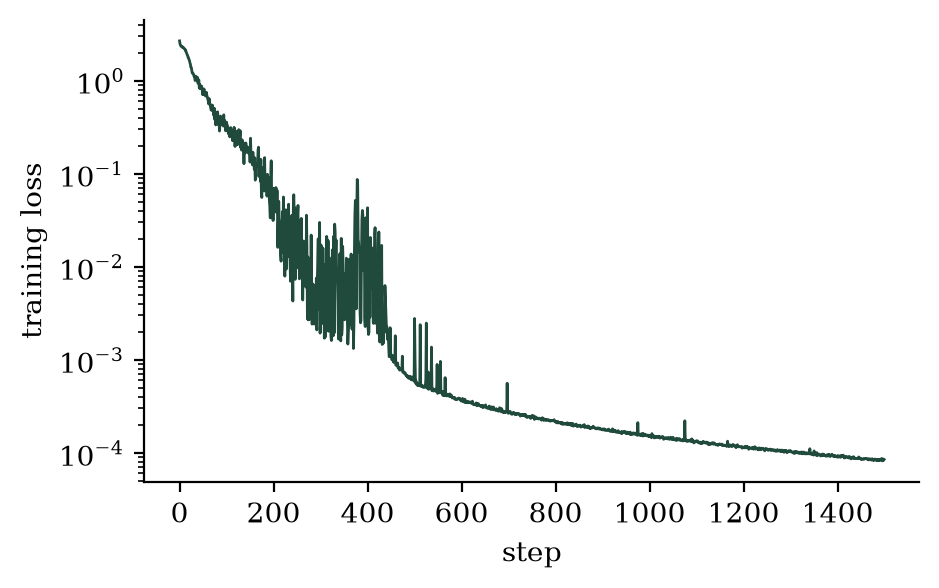
Training loss for the string-reversal model

Figure 1.1. Training loss on a log scale, one point per step. Mean loss over each block of 250 steps: 0.48, 0.0090, 0.0004, 0.0002, 0.0001, 0.0001.

The loss starts near 2.5, which is $\ln 12$, the cost of guessing uniformly over twelve tokens. It falls to around 0.01 by step 250, then spends the next 200 steps swinging between about 0.001 and 0.1, with its largest jump, to about 0.08, near step 380. After that it settles, mostly below 0.001 from about step 450 apart from brief spikes, and near 0.0001 at the end. Swings like these are common with a fixed learning rate and no warm-up; they did no lasting harm here, and chapter 4 adds the usual remedy, a warm-up followed by a decaying learning rate.

Fresh strings of the training lengths. The test draws 500 strings with lengths 3 to 8, from a different random seed than training, and decodes each one greedily: feed the letters and the separator, take the most likely next token, append it, repeat. A string counts only if every letter of the reversal is right. Result: 500 of 500. By length, 86/86, 75/75, 91/91, 106/106, 70/70, 72/72. Of the 500 test strings, 335 never appeared in training, and all 335 were reversed correctly. So the model is not reciting; on strings of length 7 and 8 it is applying something it learned to inputs it has not seen.

Longer strings. The same model was then given 200 strings of lengths 9 to 12, which it had never seen at any length. Result: 0 of 200. Asked to reverse abcdefghij, it produced fedabadbad. Generalisation across unseen strings of a familiar length is not the same thing as generalisation to lengths outside the training range, and this model has the first and not the second. Section 1.10 looks at why.

1.10 Reading the attention weights

Figure 1.2 shows the attention weights of all four heads for the input fgcabe. Each row is a query position, each column a key position, and the blank upper triangle is the mask.

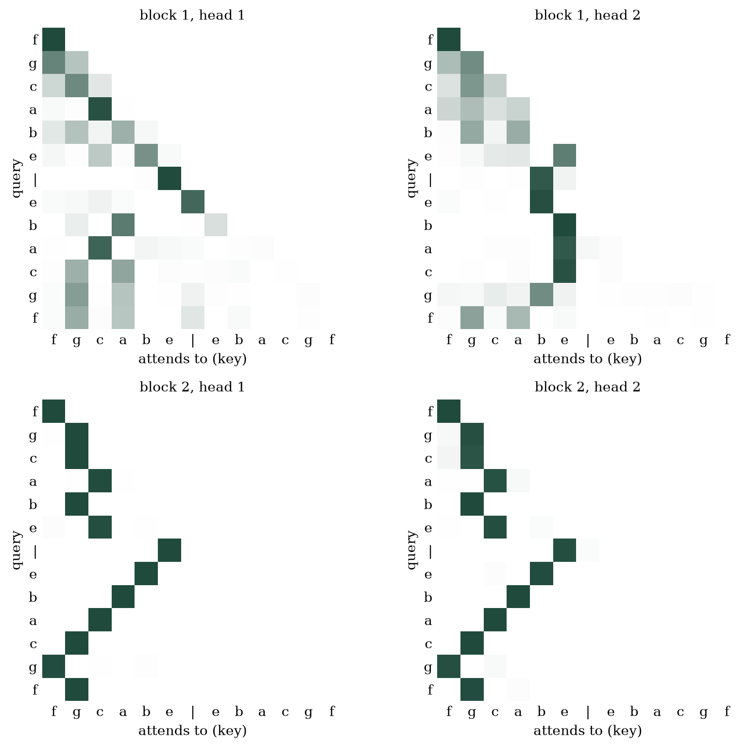
Attention weights of both blocks and both heads

Figure 1.2. Attention weights after training, for f g c a b e | e b a c g f. Darker is heavier; each row sums to one.

Start with the bottom row of plots, the second block. Below the separator, both heads put almost all of their weight on a single input letter, and the letters they pick form a diagonal running the other way. The query at | attends to e, the last input letter, which is the first letter the model has to emit. The query at the output e attends to b, the next letter it needs. Then b to a, a to c, c to g, g to f. The notebook prints the strongest key for each of these rows; the weights are between 0.97 and 1.00 in both heads. Each output position is not looking at what it just wrote. It is looking up what to write next.

That is a real finding about the model, and it is also less than it looks. Three cautions.

First, the plot shows where the weights go, not what travels. The values carry the content, the output projection mixes the heads, and the MLP that follows does whatever computation turns "I fetched the vector at this position" into "emit the letter b". None of that is visible here.

Second, the first block is doing something, and it is not this. Its heads attend to the separator, to b and e repeatedly, and to g and a in the last rows, and the pattern changes from row to row with no clean geometry. The second block's clean lookup presumably depends on what the first block wrote into each position's vector, and the plot cannot tell you what that was.

Third, the rows above the separator have no target, so nothing in the loss asks them to do anything in particular, and they do not. Unconstrained positions in a transformer usually look like that.

The attention plot is a view of one layer's information flow. It is consistent with a lookup, and the weights are as sharp as they could be, but it is not the model's reasoning laid bare.

On longer strings, the plot does not help directly, but the position table does. Rows 16 to 24 of that table received no gradient during training. Position 16 only ever holds the last letter of an 8-letter reversal, which has no target, and positions 17 to 24 only ever hold padding; no position with a target comes after them, so the mask keeps them out of every loss term, and they still hold close to their random initial values (weight decay shrank them by about 4%). Reversing a string of length 9 feeds the model 18 positions, two of which, 16 and 17, it has never learned anything about. Whether the untrained rows are the whole story is exercise 5. What the experiments notebook does show is that the same architecture, trained on lengths 3 to 12 for 3,000 steps (86 seconds), reverses all 500 test strings of lengths 9 to 12. The failure is in what the model was shown, not in what it could represent.

Where this goes wrong

All four of these were run in the experiments notebook, each a single change to the reference model. Figure 1.3 puts the training loss each run reported next to the test accuracy it reached, and the two do not agree.

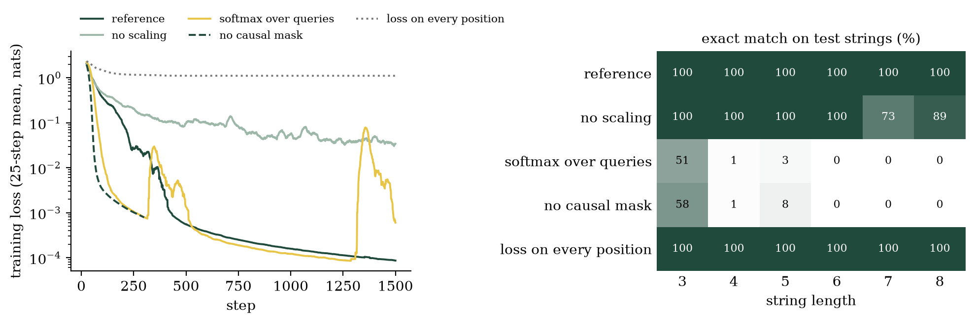
Training loss and test accuracy for the reference model and four faulty variants

Figure 1.3. Left: training loss on a log scale, 25-step mean, for the reference model and the four faults below; the run without a mask stops at 300 steps. Right: exact-match accuracy on the same 500 test strings, by string length, in percent. Two of the faulty runs reach a training loss at or below the reference's for long stretches and are nearly useless at generation time.

No scaling. Covered in section 1.4: slower learning, 94.6% instead of 100% at this width, every miss on the two longest lengths.

Softmax over the query axis. Change dim=-1 to dim=-2, keep the mask, and train. The training loss falls faster than the correct model's: the mean drops below 0.01 at step 128 instead of 362, and for most of training it sits at or below the reference's. It is also less stable, and a late jump near step 1,300 leaves the last 250 steps averaging 0.0135 (Figure 1.3). Test accuracy is 9.6%, and most of that is three-letter strings. The loss says the task is solved and the test says it is not, and both are telling the truth. With the softmax over queries, the weight that query $i$ puts on key $j$ is divided by a sum over every query $i' \geq j$, including queries later than $i$. So the weight at position $i$ depends on scores from positions after $i$. During training the whole sequence is present and that dependence leaks the answer. During generation the later positions do not exist yet, the denominators change, and the weights the model learned to rely on are gone. No weight was ever placed on a later key. The leak was in the normalisation.

No mask. Turn causal off and train for 300 steps. The mean loss is below 0.01 by step 89, because position $t$ can attend to position $t+1$, which holds the target. Exact-match accuracy at generation is 11.6%, and most of that is three-letter strings. Same shape as the previous fault: trivially low training loss, useless model. Any time the loss collapses faster than you expected, look for a leak before you celebrate.

Loss on every position. Score the input letters too. The model still reaches 100% on the test, but the loss flattens at 1.11 and stays there, because the input letters are uniformly random and cost $\ln 10 = 2.30$ per position whatever the model does; averaged with the near-zero loss on the output positions, that is about half of 2.30. The number looks like a model that has stopped learning. It is a model being asked to predict coin flips.

Exercises

Remove the division by math.sqrt(d) in attention and retrain. Record the step at which the mean loss first drops below 0.01 and compare it with the scaled run. Then change d_model to 256 and repeat both runs. What does the scaling buy, and when?
Change the softmax to dim=-2 and retrain. The training loss will fall faster than before. Then run the tests. Explain both results, and say exactly how information about later tokens reaches an earlier position in this version.
Set causal=False and train for 300 steps. The loss collapses almost immediately. Run the tests, report the exact-match accuracy, and explain why training and testing disagree.
Reduce n_layers to 1 and n_heads to 1. Train for 1,500 steps, then for 5,000. Report accuracy by string length for both runs.
The model scored zero on strings of length 9 to 12. Propose a one-line change to the training data that would let you find out whether the problem is the untrained rows of the position table or something else, run it, and report what you find.

Exercises 1 to 3 have a reference run in the experiments notebook. Exercise 5 does not, and its answer is not what I expected.

Notebooks for this chapter: 01-attention.ipynb (41 seconds of training, 55 seconds for the whole notebook) and 01-attention-experiments.ipynb (294 seconds in total), both on the laptop described at the top of the chapter. Neither downloads anything.